https://doi.org/10.5194/hess-23-2965-2019 © Author(s) 2019. This work is distributed under the Creative Commons Attribution 4.0 License.
Quantifying thermal refugia connectivity by combining
temperature modeling, distributed temperature
sensing, and thermal infrared imaging
Jessica R. Dzara1, Bethany T. Neilson1, and Sarah E. Null2
1Department of Civil & Environmental Engineering, Utah State University, 8200 Old Main Hill, Logan, Utah, 84321-8200, USA
2Department of Watershed Sciences, Utah State University, 5210 Old Main Hill, NR 210, Logan, Utah, 84321-5210, USA Correspondence:Sarah E. Null ([email protected])
Received: 17 August 2018 – Discussion started: 7 September 2018
Revised: 19 June 2019 – Accepted: 27 June 2019 – Published: 12 July 2019
Abstract. Watershed-scale stream temperature models are often one-dimensional because they require fewer data and are more computationally efficient than two- or three-dimensional models. However, one-three-dimensional models as-sume completely mixed reaches and ignore small-scale spa-tial temperature variability, which may create temperature barriers or refugia for cold-water aquatic species. Fine spatial- and temporal-resolution stream temperature moni-toring provides information to identify river features with increased thermal variability. We used distributed tempera-ture sensing (DTS) to observe small-scale stream temper-ature variability, measured as a tempertemper-ature range through space and time, within two 400 m reaches in summer 2015 in Nevada’s East Walker and main stem Walker rivers. Ther-mal infrared (TIR) aerial imagery collected in summer 2012 quantified the spatial temperature variability throughout the Walker Basin. We coupled both types of high-resolution measured data with simulated stream temperatures to cor-roborate model results and estimate the spatial distribution of thermal refugia for Lahontan cutthroat trout and other cold-water species. Temperature model estimates were within the DTS-measured temperature ranges 21 % and 70 % of the time for the East Walker River and main stem Walker River, respectively, and within TIR-measured temperatures 17 %, 5 %, and 5 % of the time for the East Walker, West Walker, and main stem Walker rivers, respectively. DTS, TIR, and modeled stream temperatures in the main stem Walker River nearly always exceeded the 21◦C optimal tem-perature threshold for adult trout, usually exceeded the 24◦C stress threshold, and could exceed the 28◦C lethal
thresh-old for Lahontan cutthroat trout. Measured stream tempera-ture ranges bracketed ambient river temperatempera-tures by−10.1 to +2.3◦C in agricultural return flows, −1.2 to +4◦C at di-versions,−5.1 to +2◦C in beaver dams, and−4.2 to 0◦C at seeps. To better understand the role of these river fea-tures on thermal refugia during warm time periods, the re-spective temperature ranges were added to simulated stream temperatures at each of the identified river features. Based on this analysis, the average distance between thermal refu-gia in this system was 2.8 km. While simulated stream tem-peratures are often too warm to support Lahontan cutthroat trout and other cold-water species, thermal refugia may ex-ist to improve habitat connectivity and facilitate trout move-ment between spawning and summer habitats. Overall, high-resolution DTS and TIR measurements quantify temperature ranges of refugia and augment process-based modeling.
1 Introduction
longi-tudinal stream temperature changes at the watershed scale but are poor predictors of thermal micro-habitats. On the other hand, high-resolution temperature monitoring provides micro-habitat information but is typically conducted over small spatial extents and thus difficult to extrapolate to the watershed scale for management and restoration decisions.
Stream temperature models are useful for river manage-ment because they help decision-makers understand stream temperature dynamics and the potential impacts of restora-tion and management. Many one-dimensional temperature models exist and have been applied to understand the temper-ature effects of dams, reservoir re-operation, climate change, and restoration in systems all over the world (e.g., Bond et al., 2015; Elmore et al., 2016; Pelletier et al., 2006). Stream temperature models used in management are often one-dimensional because they are less data intensive and more computationally efficient than two- or three-dimensional models that account for temperature variability over channel width and depth. However, one-dimensional watershed-scale models do not identify river features like cold-water pools, lateral variability, or groundwater seeps that are smaller than the model spatial resolution (Null et al., 2017).
Distributed temperature sensing (DTS) and thermal in-frared (TIR) imaging are sometimes used in conjunction with stream temperature models. DTS provides near-continuous temperature measurements in both time and space (Selker et al., 2006; Suárez et al., 2011). Raman spectra DTS is ca-pable of measuring temperatures every meter along fiber-optic cables with an accuracy of at least ±0.1◦C, and ca-bles vary between approximately 1 and 10 km (Tyler et al., 2009). DTS has determined zones of groundwater influence (Hare et al., 2015; Selker et al., 2006; Suárez et al., 2011) and hyporheic exchange (Briggs et al., 2012). DTS data were used to calibrate and validate a 1.3 km physically based, one-dimensional stream temperature model of the Boiron de Morges River in southwest Switzerland (Roth et al., 2010) and a 580 m river reach in Luxembourg’s Maisbich River (Westhoff et al., 2007). TIR imagery capture spatially con-tinuous stream surface temperatures and have successfully identified spatial heterogeneity (Bingham et al., 2012; Fuller-ton et al., 2018) and located groundwater and tributary inputs (Dugdale et al., 2013; Loheide and Gorelick, 2006; Mundy et al., 2017). However, TIR data are for a single time unless acquired on multiple occasions (Dugdale, 2016; Torgersen et al., 2001). TIR data have been used in conjunction with stationary temperature loggers to calibrate reach- and basin-scale models (Bingham et al., 2012; Cardenas et al., 2014; Carrivick et al., 2012; Deitchman and Loheide, 2012). For example, TIR data were combined with instream tempera-ture loggers to calibrate an 86 km QUAL2Kw water qual-ity model in the Wenatchee River in Washington (Cristea and Burges, 2009) and a 100 km statistical model in the Big Hole River, MT, USA (Vatland et al., 2015). In the latter study, Vatland et al. (2015) concluded that point monitoring sites underestimate the temporal and spatial heterogeneity in
stream temperatures and that DTS data would be a promising addition to TIR and stationary loggers.
Recent research has quantified when and where fish use thermal refugia, although results are system or species spe-cific. For example, in the Pacific Northwest and northern Cal-ifornia, thermal refugia are generally 2.7–13 km long and are spaced approximately 5.7–49.4 km apart using TIR data with spatial resolution of at least 250 m (Fullerton et al., 2018). Authors emphasized that this is the existing refugia distri-bution, not necessarily the distribution that is needed to sup-port migratory fish. In northeastern Oregon, doubling the fre-quency of thermal refugia increased the abundance of rain-bow trout and Chinook salmon, while doubling refuge area had only minor improvements for rainbow trout abundance (Ebersole et al., 2003). Brewitt and Danner (2014) showed that 80 % of juvenile steelhead trout in the Klamath River move into refuges when stream temperatures are 22–23◦C,
and all move when stream temperatures exceed 25◦C.
Sim-ilarly, adult Atlantic salmon in Canada’s Quebec River ther-moregulate body temperature by using large, stratified pools with temperatures of 17–19◦C (Frechette et al., 2018). In Idaho’s North Fork Coeur d’Alene River, westslope cutthroat trout that were larger than 300 mm used side channels that were cooler than 20◦C and deeper than 2 m, although smaller fish were less likely to use thermal refugia (Stevens and DuPont, 2011). Brook char that leave cool water refugia for less than 60 min to forage maintained body temperatures be-low critical thresholds in laboratory experiments. Thus, short excursions allowed fish to forage during long periods of un-favorable stream temperatures (Pépino et al., 2015). To date, no studies have used DTS and TIR to quantify temperature ranges by river feature within model reaches and use that in-formation to estimate likely temperature ranges over space and time at the watershed scale. Such insight into micro-habitats allows researchers, managers, and stakeholders to identify thermal refugia and estimate potential temperature ranges by river feature.
2 Study site
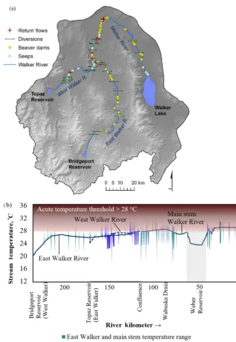
The Walker River flows from the east-slope Sierra Nevada Mountains into Walker Lake, a terminal lake in the Great Basin (Fig. 1). The lower elevations of the Walker Basin have an arid climate with hot summers, whereas high elevations receive heavy snowfall during cold winters (Sharpe et al., 2008). The Walker River is a desert stream with annual flow of 15.5–30 m3s−1, mean width of approximately 7.6 m and depth of about 33 cm. The main stem Walker River is the con-fluence of two branches, the East Walker River and the West Walker River. In the prolonged drought of 2011–2017, lower portions of the Walker River were dry and disconnected from Walker Lake in fall of 2014 and 2015 (Null et al., 2017).
Agriculture is the main land use in the basin. Irri-gated farmland makes up approximately 450 km2 of the 10 720 km2 Walker Basin (Sharpe et al., 2008). Bridgeport Reservoir on the East Walker River, Topaz Reservoir on the West Walker, and Weber Reservoir on the main stem Walker River regulate water to support agriculture and other human water uses. There are 23 diversions and 8 return flows in the East, West, and main stem Walker rivers, which influence both streamflows and stream temperatures. The Walker River generally gains water during wet years and loses flow during dry years (Carroll et al., 2010). Agricultural flood irrigation replenishes groundwater levels during the summer months (Carroll et al., 2010; Lopes and Allander, 2009).
Walker Lake once supported healthy populations of La-hontan cutthroat trout (LCT) (Oncorhynchus clarkii hen-shawi), which spawned in the Walker River and tributaries. The historic range of LCT is the Lahontan Basin in east-ern California, southeasteast-ern Oregon, and northeast-ern Nevada, although LCT persist in less than 10 % of their historic range because they are limited by warm stream temperatures, low streamflows, and low dissolved oxygen (Coffin and Cowan, 1995; USFWS, 2003). LCT are now listed as a threatened species under the Endangered Species Act (USFWS, 1975). Field studies conducted in Coyote Lake (Oregon), Quinn River (Oregon and Nevada), and Humboldt River (Nevada) indicate LCT occurrence is reduced at stream temperatures above the acute (<2 h) threshold of 28◦C (Dunham et al., 2003). Measured main stem Walker River stream temper-atures exceeded the acute 28◦C temperature threshold for LCT throughout summer in 2014 and 2015, demonstrating that warming stream temperatures are a concern for LCT in the Walker Basin (Null et al., 2017).
Low instream flows from surface water diversions have caused the Walker Lake level to decline, increasing dissolved salts in the lake to concentrations which do not support trout and native benthic insects (Herbst et al., 2013; Wurtsbaugh et al., 2017). To address these problems, an environmental water purchase program acquires natural flow and storage water rights from willing sellers who switch to crops that re-quire less water or improve agricultural water use efficiency (NFWF, 2018; Walker Basin Conservancy, 2018). To date,
2.3 m3s−1 of natural flow water rights and 13.3 million m3 of storage water rights have been purchased, approximately 40 % of the water needed to restore Walker Lake salinity to tolerable levels (Walker Basin Conservancy, 2018). Pre-vious modeling has suggested that environmental water pur-chases intended to increase lake elevation also improve habi-tat conditions for LCT and other aquatic biota in the Walker River by increasing streamflows, reducing stream tempera-tures, and increasing dissolved oxygen concentrations (El-more et al., 2016; Null et al., 2017).
3 Methods
3.1 Distributed temperature sensing (DTS) data 3.1.1 DTS data collection
DTS units measure temperatures by sending a laser pulse down a fiber-optic cable and timing the return signal. Al-though most of the reflected energy has its original wave-length, a portion of the energy is absorbed and re-emitted at both shorter (anti-Stokes backscatter) and longer (Stokes backscatter) wavelengths. Temperatures along the cable are determined from the Stokes/anti-Stokes ratio (Selker et al., 2006). A 1 km silver armored DTS cable was deployed to measure diurnal stream temperatures in the main stem and East Walker rivers. Data were collected over 400 m in the East Walker River at Rafter 7 Ranch on 18–23 June 2015 and over 450 m in the main stem Walker River at Stanley Ranch on 25–30 June 2015 (Fig. 1). The year 2015 was dry and the snowpack was at 5 % of normal levels. The DTS ca-ble was deployed in a U shape at both sites, with approxi-mately 400 m of cable on each side of the stream to capture lateral stream temperature differences. The cable was sus-pended in the water column approximately 10 cm above the streambed with steel stakes and leashes. Main stem Walker River DTS deployment included approximately 20 m of a flood irrigation return flow canal named the Wabuska Drain. The Wabuska Drain was not flowing during the drought when the DTS was deployed but contained standing water and was connected on the surface with the Walker River.
A two-channel Sensornet Orxy DTS unit measured stream temperatures at a spatial resolution of 1 m and temporal res-olution of 15 min. Each data collection event measured tem-peratures over 30 s and averaged temperature over the 1 m spatial interval. Measurement precision from the unit was 0.01◦C in the −40 to 65◦C range. The DTS had two
co-located fibers within the cable producing two single-ended datasets.
thermocou-Figure 1.Walker River modeled extent, June 2015 DTS deployment sites, and July 2012 TIR imagery extent.
ple temperature sensors that are accurate to 0.002◦C in the −5 to 35◦C range measured calibration bath temperatures. Nine Maxim Integrated iButton thermistors provided addi-tional stream temperature measurements along the cable ev-ery 15 min to verify DTS temperatures. iButton temperature loggers are accurate to 0.5◦C in the−40 to 85◦C range. Cal-ibration used a linear transformation to correct the DTS data based on the difference between the DTS and thermocou-ple temperatures. Post-collection processing used the single-ended explicit calibration method developed by Hausner et al. (2011). Due to cable damage near the splice box prior to the third calibration bath, postprocessing relied upon iBut-ton data closest to the end of the cable and the two calibra-tion bath thermocouples near the DTS. Seccalibra-tions of cable that were exposed to air were removed from the dataset. Data points were also removed if the temperature difference be-tween the two single-ended datasets was>1◦C because ten-sion on the DTS cable can result in erroneous temperature measurements (Hausner et al., 2011). Temperatures for these points were linearly interpolated between the upstream and downstream cable locations. We reported the average root mean square error (RMSE) of the two thermocouples and iButton to quantify DTS error for the length of the cable for each single-ended dataset. The single-ended dataset with
the lowest calibrated RMSE was used for data analysis and results. In addition, RMSE was calculated between georefer-enced iButton stream temperature measurements and the cor-responding georeferenced DTS stream temperature measure-ments for the data collection period to provide additional cor-roboration of the DTS temperatures. iButton residuals were calculated as the difference between iButton temperatures and co-located DTS-measured temperatures.
[image:4.612.127.469.66.390.2]1.0 m3s−1 (36 ft3s−1) in the Walker River during deploy-ment (Fig. S2).
3.1.2 DTS data analysis
DTS minimum (Tmini,s), maximum (Tmaxi,s), and
site-averaged stream temperatures (Ti,s) were calculated for each DTS sample event,i, at each DTS site,s(Table 1). Similarly, minimum (Tminp,s) and maximum (Tmaxp,s) stream
tempera-tures for the deployment period, p, at each DTS site were calculated. Deployment period average temperatures (Tp,s) were calculated from the spatial average of each sampling event, which occurred every 15 min, following Eq. (1):
Tp,s= t P
i=1
Ti,s
p . (1)
The temperature range of each DTS sample event at a de-ployment site (Ri,s) was calculated by subtracting the min-imum measured temperature (Tmini,s) from the maximum
measured temperature (Tmaxi,s) for the 1000 m DTS cable.
The minimum (Rminp,s) and maximum (Rmaxp,s) temperature
range during the deployment period for each deployment site were also calculated. The deployment period average DTS stream temperature range (Rp,s) was calculated from the sample events for each DTS site following Eq. (2):
Rp,s= t P
i=1
Tmaxi,sTmini,s
p . (2)
Left and right river bank temperatures represent lateral ther-mal variability and were estimated from DTS data at 1, 10, 100, and 300 m extents to quantify thermal variability over multiple spatial scales. Lateral variability was evaluated for the hottest sample time during each DTS deployment in the main stem Walker and East Walker rivers. For the 1 m com-parison, we used left and right bank measurements perpen-dicular to the thalweg. At larger spatial scales, we compared the minimum and maximum temperatures for each bank for 10, 100, and 300 m extents. The temperature range at each scale was then estimated as the maximum absolute value of the difference between the two banks. Wabuska Drain was not included in these analyses.
3.2 Airborne thermal infrared (TIR) data 3.2.1 TIR data collection
TIR imagery of the Walker River was collected by Water-shed Sciences Inc. on 16–17 November 2011 (winter flight) and 18 and 24–26 July 2012 (summer flight) (Watershed Sci-ences Inc., 2011, 2012). We used summer TIR data for all analyses in this paper, except to identify possible cool-water seeps, which were more apparent with the winter dataset. The
year 2012 was dry year and the snowpack was at 50 % of nor-mal levels. TIR flights measured surface stream temperatures for 240 river kilometers in the East Walker, West Walker, and main stem Walker rivers to Weber Reservoir (Fig. 1). Stream temperatures warmed by 1 to 2◦C (average 1.6◦C) between 14:00 and 16:00 LT (local time) when TIR data were col-lected. A FLIR Systems, Inc. SC6000 sensor (wavelength of 8–9.2 µm, Noise Equivalent Temperature Differences of 0.035◦C, and pixel array of 640×512 at a 14 bit encoding level) mounted on the underside of a Bell Jet Ranger He-licopter collected imagery and was flown at an altitude of approximately 610 m. Pixel resolution was 0.6 m (Watershed Sciences Inc., 2012).
Watershed Sciences Inc. calibrated and georeferenced the data and provided raster layers of the data. Tribu-tary inflow temperatures were reported at their confluence with the Walker River. Watershed Sciences, Inc. also pro-vided summary point data, which are minimum, median, and maximum temperatures of 10 pixels from the middle of the stream. Flight speed, image overlap, and river fea-tures determined which images to sample (Watershed Sci-ences Inc., 2012). We used georeferenced TIR rasters and summary points for analyses. TIR data were collected on warm summer days with low humidity. Average air temper-ature during data collection was 33.1◦C and average wind speed was 11.6 km per hour (kph) in Yerrington, NV. Aver-age flow during data collection was 1.0 m3s−1 (34 ft3s−1), 1.1 m3s−1 (39 ft3s−1), and 2.8 m3s−1 (100 ft3s−1) in the main stem Walker River (USGS gage 10301500), West Walker River (USGS gage 10298600), and East Walker River (USGS gage 10293500), respectively (Watershed Sciences Inc., 2012). Calibrated TIR radiant temperatures were vali-dated with 28 Hobo Pro and iButton sensors. See Watershed Sciences Inc. (2012 and 2011) for additional TIR data col-lection details.
3.2.2 TIR data analysis
To compare measured TIR surface temperatures with model results, TIR summary points provided by Watershed Sci-ences Inc. (2012) were georeferenced with the 300 m mod-eled reaches. On average, there were three TIR summary points per 300 m modeled reach. The spatial averages of min-imum, maxmin-imum, and median TIR temperature were cal-culated for the East Walker, West Walker, and main stem Walker rivers.
Table 1.Description of DTS stream temperature variables.
Variable Metric Temporal extent (t) Spatial extent
Tmini,s Minimum temperature of sample event 30 s sample event
Tmaxi,s Maximum temperature of sample event occurring every 15 min (i)
Ti,s Average temperature of sample event Tminp,s Minimum temperature of deployment period
Tmaxp,s Maximum temperature of deployment period Deployment period (p)
Tp,s Average temperature of deployment period Deployment site (s) Ri,s Temperature range of sample event 30 s sample event
(Tmaxi,s−Tmini,s) occurring every 15 min (i)
Rminp,s Minimum temperature range of deployment period
Rmaxp,s Maximum temperature range of deployment period Deployment period (p)
Rp,s Average temperature range of deployment period
3.3 River Modeling System (RMS) modeled stream temperatures
Previous research provided modeled streamflows and stream temperatures for one wet (2011) and three dry (2012, 2014, 2015) 1 April–31 October irrigation seasons using River Modeling System (RMS) (Elmore et al., 2016; Null et al., 2017). RMS is a one-dimensional hydrodynamic and water quality model which solves the St. Venant equations for con-servation of mass and momentum and the Holly–Priessmann mass transport equation (Hauser and Schohl, 2002). Input re-quirements for the hydrodynamics module are channel ge-ometry, roughness coefficients, boundary condition stream-flow, and initial surface water elevations. Outputs are veloc-ity and depth at each model node which are passed to the water quality module. Additional inputs for the water qual-ity module include weather data, riparian shading estimates, boundary temperatures, and initial water temperature. Water quality outputs are hourly stream temperatures (Hauser and Schohl, 2002).
The RMS model was developed to simulate stream tem-peratures from environmental water purchases that alter ther-mal mass. Irrigation season was modeled because it is the time period that environmental water purchases occur from irrigators. A total of 305 river kilometers were represented in RMS at an hourly time step. Model reaches over the model extent were 300 m. As a one-dimensional model, each reach was completely mixed and had a homogenous temperature. Walker River modeled extent included the East Walker River downstream of Bridgeport Reservoir (river kilometers 243 to 117), the West Walker River downstream of Topaz Reser-voir (river kilometers 60 to 0) and the main stem Walker River to Walker Lake (river kilometers 117 to 0) (Fig. 1). For additional model details see Elmore et al. (2016) and Null et al. (2017).
3.4 Comparison of measured and modeled data
We calculated the percentage of time that the model over-or underpredicted DTS temperatures and the percentage of space that the model over- or underpredicted TIR tempera-tures to quantify the thermal range not captured within one-dimensional modeling. We used hourly, spatially averaged DTS measurements and omitted Wabuska Drain tempera-tures to compare DTS data to model results. TIR data were averaged for 300 m reaches to compare with model results. RMSE, mean absolute error (MAE), and mean bias summa-rized differences between modeled and measured data.
The percentage of time that DTS and modeled stream tem-peratures were below 21, 24, and 28◦C and the river
ex-tent that TIR and modeled stream temperatures were below the same thresholds were also calculated. Temperatures be-low 21◦C are optimal for adult LCT (Hickman and Raleigh, 1982), temperatures exceeding 24◦C are stressful for LCT (Dickerson and Vinyard, 2003), and temperatures exceeding 28◦C are lethal for LCT (Dunham et al., 2003).
were dry during the summer flight (Watershed Sciences Inc., 2011, 2012). However, we quantified the observed tempera-ture variability at seeps using the summer 2012 TIR flight (Watershed Sciences Inc., 2012). Beaver are native to the Walker Basin (Gibson and Olden, 2014) and beaver dams were identified using 2012 and 2013 Google Earth aerial im-agery (Google Earth Pro, 2018). We included beaver dams that spanned the channel. Often turbulence was observed be-low the dam and sometimes crowdsourced photos added im-ages of the beaver dams from the ground. We relied primar-ily on 2012 imagery, unless it was unavailable or of poor quality, when 2013 aerial imagery was used. Both 2012 and 2013 were dry years, and beaver dams are more abundant in the Walker River during dry years, when high flow events that limit beavers’ ability to dam across the stream channel are reduced (Nevada Department of Wildlife, 2016). Using this information, we then added or subtracted measured tem-perature ranges to modeled temtem-peratures at each of the geo-referenced river features to provide an estimate of the ther-mal variability occurring at sther-mall spatial scales not captured by the one-dimensional model predictions.
4 Results
4.1 DTS stream temperatures and ranges
Average RMSE between calibrated DTS data and the three reference temperatures was 0.09 and 0.15◦C for the East Walker River and main stem Walker River DTS sites, respec-tively (Table S1 in the Supplement). Average DTS error for both sites was also within the 0.5◦C precision of the iBut-tons. There were no significant residual trends in errors for the main stem Walker River (Table S2 and Fig. S1 in the Supplement).
DTS temperatures in the East Walker River changed more through time than through space (Fig. 2). The deployment period minimum stream temperature (Tminp,s) was 16.7
◦C,
maximum temperature (Tmaxp,s) was 24.9
◦C, and average
stream temperature (Tp,s) was 21◦C (Table 2). Maximum temperatures were measured in a straight, homogenous, un-shaded section (Fig. 3). The stream temperature range for each DTS collection event (Ri,s) varied from a minimum of 0.5◦C to a maximum of 2.0◦C for the deployment pe-riod, with an average (Rp,s) of 1.0◦C. A shaded backwa-ter eddy and pools with overhanging shrubs and tall cot-tonwoods were river features with increased thermal hetero-geneity in the East Walker River (Fig. 3).
Stream temperatures varied spatially throughout the main stem DTS site, visualized as color striations in Fig. 2b. Av-erage deployment site temperature (Tp,s) was 25.2◦C, not including the Wabuska Drain segment (Table 2, excluding distance 110–175 m in Fig. 2b). Maximum stream temper-ature (Tmaxp,s) was 32.9
◦C. The average temperature range
for the deployment (Rp,s) was 2.7◦C, with a minimum
de-Figure 2.Stream temperatures measured for the length of the DTS cable at East Walker River(a)and main stem Walker River(b)DTS sites. Wabuska Drain, which was not flowing but had standing water during sampling, is located at cable distance 110–175 m in the main stem Walker River site.
ployment site temperature range (Rminp,s) of 1.1
◦C and a
maximum site temperature range (Rmaxp,s) of 7.0
◦C.
Aver-age DTS stream temperatures (Tp,s) in the East Walker River were approximately 4◦C cooler and less variable than the main stem Walker River (Fig. 2). Average DTS tempera-ture ranges (Rp,s) were nearly 2◦C greater in the main stem Walker River than the East Walker River. The East Walker River DTS site is farther upstream and close to Bridgeport Reservoir, a bottom release dam. The main stem Walker River DTS site is 92 km downstream from the East Walker River DTS site and receives contributions from the West Walker River, which is fed by surface water releases from Topaz Reservoir.
[image:7.612.311.543.69.416.2]Figure 3.East Walker River daily maximum stream temperatures on 21 June 2015. Insets show details of spatial temperature variability. Modeled reach points represent the division between 300 m modeled reaches.
Drain. However, the maximum temperature range during the deployment (Rmaxp,s) increased considerably from 7.0 to
10.2◦C and the average temperature range for the deploy-ment (Rp,s) also increased from 2.7 to 3.6 ◦C (Table 2, Fig. 2b). Figure 4 illustrates cooler temperatures in the Wabuska Drain during most times and spatial temperature variability during daily maximum stream temperatures on 29 July. The coolest temperature (Tmini,s) at that time in the
main stem Walker River DTS site was 24.4◦C and occurred approximately 20 m into Wabuska Drain (Fig. 4). Stream temperatures of up to 31.8◦C (T
maxi,s) occurred in the
ho-mogeneous main stem Walker River segment just upstream of the Wabuska Drain along the shallow right bank and at the mouth of the drain. The shallow Wabuska Drain also experi-enced rapid heating and cooling in response to atmospheric conditions. Cool water from the outlet of the Wabuska Drain mixed with the main stem Walker River at hot times of day, expanding the temperature range downstream of the drain. In addition to wider temperature ranges in the Wabuska Drain, the main stem Walker River had greater temperature hetero-geneity from inactive, breached beaver dams. On 29 June at 15:15 LT, when average site temperature (Ti,s) was 29.6◦C
for this sample event, nearly 7◦C of temperature range ob-served for this event occurred at a breached beaver dam (Fig. 4).
Figure 4.Main stem Walker River daily maximum stream temperature on 29 June 2015. Model reach points represent the division between 300 m model reaches.
4.2 TIR stream temperatures and ranges
TIR data were within 0.5◦C of iButton sensors, except for one location in the East Walker River where redundant sen-sors were 1.7 and 3.3◦C cooler than radiant TIR temperature,
and one location in the West Walker River where an iButton was 1.1◦C cooler than radiant TIR temperature. TIR mea-sures water surface temperatures, so these discrepancies may have occurred where the river was not well mixed.
While DTS measurements provided high spatial and tem-poral stream temperature resolution at two sites, TIR mea-surements provided continuous stream surface temperatures throughout the Walker River for a single time. Maximum
stream temperatures typically occurred in reaches with canal diversions and return flows. The warmest temperature in the East Walker River (Table 3) was 26.5◦C where water ponds
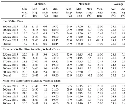
Table 2.Daily stream temperatures and ranges for DTS deployments in the East Walker River (11:15 LT on 19 June 2015 to 09:45 LT on 23 June 2015) and main stem Walker River (14:15 LT on 25 June 2015 to 12:30 LT on 30 Jun 2019).
Minimum Maximum Average
Min. Min. Min. Min. Max. Max. Max. Max. Avg. Avg.
temp. temp. range range temp. temp. range range temp. range (◦C) time (◦C) time (◦C) time (◦C) time (◦C) (◦C)
East Walker River
19 June 2015 19.8 11:15 0.6 19:45 24.9 17:00 1.4 13:00 23.1 1.0 20 June 2015 18.0 06:15 0.5 08:30 24.9 17:30 2.0 13:00 21.3 1.1 21 June 2015 18.0 06:15 0.5 23:30 24.4 17:30 1.5 13:45 21.2 0.9 22 June 2015 16.7 08:30 0.5 00:30 24.0 17:30 1.7 14:45 20.3 1.0 23 June 2015 17.3 08:00 0.5 08:15 21.0 00:15 1.1 09:45 18.9 0.7
Overall 16.7 08:30 0.5 08:15 24.9 17:00 2.0 13:00 21.0 1.0
Main stem Walker River including Wabuska Drain
25 June 2015 22.0 14:15 3.6 23:45 32.9 16:15 10.2 16:00 28.6 7.1 26 June 2015 21.0 06:30 1.6 23:00 29.9 14:15 6.5 14:15 25.0 3.8 27 June 2015 21.8 07:00 1.4 09:15 31.0 15:45 6.7 15:45 25.8 3.0 28 June 2015 21.8 08:00 1.4 09:30 26.9 16:30 3.2 16:30 24.3 2.2 29 June 2015 21.0 06:00 2.0 08:30 31.9 15:15 7.5 15:15 25.2 3.7 30 June 2015 20.0 06:45 2.4 10:00 29.5 12:30 6.3 12:30 23.1 3.5 Overall 20.0 06:45 1.4 09:30 32.9 16:15 10.2 16:00 25.2 3.6
Main stem Walker River excluding Wabuska Drain
25 June 2015 23.7 23:45 2.2 19:15 32.5 16:15 7.0 15:30 28.8 3.9 26 June 15 20.0 06:30 1.2 21:00 29.9 14:15 4.5 14:00 25.1 2.5 27 June 2015 21.8 07:00 1.1 09:30 31.0 15:45 3.4 15:45 25.8 1.8 28 June 2015 21.8 08:00 1.2 09:30 26.9 16:30 3.1 15:45 24.4 2.0 29 June 2015 21.0 06:00 1.8 09:45 31.9 15:15 7.0 14:00 25.3 3.5 30 June 15 20.0 06:45 2.3 10:00 29.5 12:30 5.7 12:30 23.1 3.4
Overall 20.0 06:45 1.1 09:30 32.5 16:15 7.0 15:30 25.2 2.7
Drain (Fig. 5). This may be due to groundwater inflows downstream of the Wabuska Drain consistent with valley nar-rowing (Watershed Sciences Inc., 2012) or shallow ground-water contributions due to irrigation of adjacent fields. While groundwater interactions may have been less obvious when the return canal was flowing, DTS results showed evidence of cool water inputs when the canal was not flowing. Thus, monitoring suggests that large diversions and return flows can create warm water conditions when active, but they may also recharge shallow aquifers, increase shallow groundwa-ter contributions, and create pockets of cold wagroundwa-ter. Shallow subsurface contributions to Wabuska Drain may not occur when groundwater levels decline outside of irrigation season (Naranjo and Smith, 2016).
The 300 m reaches with the greatest temperature ranges corresponded to locations of canal diversions, return flows, and groundwater seeps (Fig. 6). In the East Walker River, the Fox–Mickey Diversion (river kilometer 126) and Stros-nider Diversion (river kilometer 140) had large tempera-ture ranges. In the main stem Walker River, thermal vari-ability occurred at the Spragg–Alcorn–Bewley Diversion
Table 3.Stream temperatures and temperature range within 300 m modeled reaches by river from July 2012 TIR data.
Min. Max. Avg. Max. Avg.
temp. temp. temp. range range
(◦C) (◦C) (◦C) (◦C) (◦C)
East Walker River 20.1 26.5 24.7 1.1 0.3
West Walker River 24.1 27.1 25.6 1.2 0.4
Main stem Walker River 22.9 29.2 27.3 1.0 0.3
[image:10.612.307.546.496.568.2]Figure 5.TIR raster data of the main stem Walker River near the Wabuska Drain with 50 and 300 m buffers.
Comparing minimum TIR stream temperatures at 50 and 300 m reaches improves understanding of thermal refugia at multiple spatial scales. We did not calculate temperature ranges because mixed pixels that contained water and land areas resulted in high maximum temperatures, and thus tem-perature ranges. We discuss this further in the limitations section. Overall, absolute minimum stream temperatures for each river were identical for 50 m and 300 m reaches, and were 21◦C for the East and West Walker rivers and 22.3◦C for the main stem Walker River. However, minimum tem-peratures varied among 50 m river segments that made up each 300 m river segment (Fig. 5). Thus, average minimum temperatures were 0.8◦C warmer when analyzing data at the 50 m scale than the 300 m scale. This highlights the extent to which spatial temperature variability varies by the scale of analysis.
4.3 RMS predictions vs. measured temperatures Modeled versus DTS stream temperature RMSE was 1.1◦C in the East Walker River and 1.7◦C in the main stem Walker
River (Table 4). When compared to TIR data, RMSE and bias were both<1◦C for the East and West Walker rivers. How-ever, RMSE in the main stem Walker River was 3.4◦C and bias was −2.5◦C, where the model performed poorly un-der low flow conditions (Table 4). Main stem Walker River TIR versus modeled stream temperature was the only RMSE value that exceeded the calibrated RMS model RMSE of 2.5◦C (Null et al., 2017). Model bias for the East Walker
River indicated the model overestimated stream temperature by 0.2◦C in the DTS site over the 5 d study period and
un-derestimated temperature by 0.5◦C for the 77 km TIR extent.
In the main stem Walker River, the model underestimated stream temperatures by 0.4◦C from the average DTS val-ues and underestimated stream temperatures by 2.5◦C when compared to the TIR data (Table 4).
Modeled temperatures in 2015 were warmer than DTS maximum hourly temperatures 50 % of the time in the East Walker River and 20 % of the time in the main stem Walker River. Conversely, the model underpredicted DTS tempera-tures 29 % and 10 % of the time in the East Walker and main stem Walker rivers, respectively (Table 4, Fig. 7a and b). Temperatures measured in Wabuska Drain were excluded from this analysis because the model simulated tures in the main channel only. Simulated 2012 tempera-tures were colder than TIR summary point minimum temper-atures for 74 %, 95 %, and 87 % of survey extent in the East Walker, West Walker, and main stem Walker rivers, respec-tively (Fig. 7c–e, Table 4). Stream temperatures in the lower Walker River could be 4–6◦C warmer than model predic-tions. That reach had challenging conditions for simulation models with a wide channel and low flow conditions. 4.4 Thermal habitat and thermal refugia connectivity Stream temperatures were rarely cooler than 21◦C, and this finding was consistent among the DTS, TIR, and modeled data (Table 5). An exception was during the East Walker River DTS deployment in June 2015, when nearly 50 % of DTS samples and modeled results were below 21◦C. Of the TIR, DTS, and RMS model datasets evaluated, stream tem-peratures were most likely to exceed 28◦C based on
condi-tions captured in the TIR dataset. Nearly all TIR and mod-eled temperatures for the West Walker River were between 24 and 28◦C in July 2012. However, with all datasets, the main stem Walker River nearly always exceeded 21◦C, usu-ally exceeded 24◦C, and could exceed 28◦C. TIR stream temperature measurements in the lower reaches of the main stem Walker River remained near the LCT lethal tempera-ture threshold for an additional 45 km than was previously estimated using the temperature model.
Figure 6.Temperature range within each 300 m model reach from July 2012 TIR summary point data.
Table 4.RMSE, MAE, mean bias, and percent of modeled dataset outside of measured values for the East, West, and main stem Walker rivers between hourly modeled, DTS, and TIR stream temperatures.
RMSE MAE Mod.– Mod.> Mod.< n (◦C) (◦C) meas. meas. meas. (h)
bias (%) (%)
(◦C)
East Walker River DTS 1.1 0.9 0.2 50 29 94
Main stem Walker River DTS 1.7 1.3 −0.4 20 10 118
East Walker River TIR 0.8 0.6 −0.5 9 74 2
West Walker River TIR 0.9 0.8 −0.8 0 95 1
Main stem Walker River TIR 3.4 2.7 −2.5 8 87 3
[image:12.612.135.459.580.702.2]Figure 7.Hourly minimum and maximum DTS site temperatures compared to model predictions in the East Walker River(a)and main stem Walker River(b)(Wabuska Drain temperatures are not included as they were not modeled). July 2012 minimum and maximum TIR temperatures calculated for every 300 m model reach length compared to modeled temperatures for East Walker(c), West Walker(d), and main stem Walker(e)rivers. The upstream end of Weber Reservoir is river kilometer 48. The river flows from left to right in(c–e). Shaded region shows temperatures exceeding the 28◦C lethal threshold for LCT.
DTS and TIR temperature variability to model results indi-cates that cool-water refugia may sometimes exist to support species migration between Walker Lake and tributaries of the Walker River (Fig. 8b). The shortest distance between refugia, or cooler pockets of water, was 0.3 km, which was the spatial resolution of model reaches. The maximum dis-tance between refugia was 37 km and occurred near Weber Reservoir in the main stem Walker River. The mean distance between refugia was 2.8 km and the median distance was 0.9 km.
5 Limitations
Figure 8.Locations of river features that affect stream temperatures in the Walker Basin(a). Daily maximum RMS stream temperatures for 29 June 2015 with estimated temperature variability by river feature using daily maximum DTS data from 29 June 2015 and TIR data from 2012(b).
et al., 2010). Field crews used leashes to secure the DTS ca-ble, which was monitored daily to minimize stress and drift. We deployed the DTS during mid-summer when we antic-ipated stream temperatures would be warm as a worst-case scenario for thermal habitat. Additional research is needed to quantify how results would change when the Wabuska Drain is flowing, or for deployments earlier or later in summer.
Table 5.Percentage of DTS, TIR, and RMS model stream temper-atures that exceed 21, 24, and 28◦C temperature thresholds.
>21◦C >24◦C >28◦C
Main stem Walker River
DTS 98.6 62.4 17.3
Modeled DTS collection period 100 64.4 6.8
TIR 100 98.7 47.2
Modeled TIR collection period 100 77.1 0
East Walker River
DTS 51.0 7.3 0
Modeled DTS collection period 54.3 13.8 0
TIR 99.2 93.7 23.5
Modeled TIR collection period 99.0 54.6 0
West Walker River
TIR 100 99.9 24.7
Modeled TIR collection period 100 100 0
2016). Clipping TIR data to the stream channel was impre-cise for datasets collected over large spatial extents. If pixels included stream banks or vegetation, they skewed calcula-tions. For this reason, we did not report maximum temper-atures of pixels within 50 or 300 m reaches, nor could we report temperature ranges which relied upon maximum tem-perature pixels. We assumed a vertically mixed water col-umn when analyzing the DTS and TIR data. Pools and beaver dams may stratify vertically, increasing the local temperature variability from what was measured or predicted. Quantify-ing temperature range from vertical stratification was outside the scope of this paper.
Obtaining small-scale spatial and temporal stream temper-atures and comparing them to model results has several limi-tations. First, resolution varied between DTS, TIR, and mod-eled data, reducing the number of comparable observations. TIR imagery represents a single point in time unless flights are repeated. DTS measurements were dense (1 m in these deployments with a 15 min temporal resolution) but were limited by cable length and field crews to monitor the deploy-ment. Second, DTS and TIR measurements were collected in different years because we used existing TIR imagery col-lected as part of the Walker Basin Project, a multipartner ef-fort to sustain the basin’s economy, ecosystem, and lake. Fu-ture studies could collect data specifically to overlap in time and space so that temperature distributions along the river are not affected by different years and sample periods. However, opportunistically using existing data for reanalysis and to im-prove model result interpretation and river management is a laudable goal that may reduce the cost of river science and management. Multiyear and multipartner river monitoring, modeling, and management is common in large, important, or complex river basins. This research highlights the
differ-ences in temperature variability given alternative sampling and modeling methods.
6 Discussion
We measured small-scale stream temperature variability that was unquantified in an existing one-dimensional, basin-scale model. Overall, DTS measured a larger maximum temper-ature range than TIR imagery in the East Walker River (2.0 and 1.1◦C, respectively) and main stem Walker River (10.2 and 1.0◦C, respectively) (Tables 2 and 3) because DTS could measure temperatures that varied spatially within the water column and over short distances where beaver dams or return flows existed. The warmest temperatures were mea-sured by TIR in the East Walker River (26.5◦C), but by DTS in the main stem Walker River (32.9◦C), indicating that these
methods complement each other, but also suggesting that different years may result in alternate temperature distribu-tions along the river (Tables 2 and 3). DTS and TIR augment process-based modeling by identifying river features that may provide thermal refugia. The range of temperatures in river features like seeps, beaver dams, diversions, and return flows were added to simulated temperatures to estimate ther-mal refuge distribution throughout the watershed. Coupling high-resolution stream temperature monitoring with process-based modeling results in a more realistic stream temperature range than one-dimensional modeling alone, especially when model results assess habitat suitability to identify promising restoration strategies and watershed-scale management.
Temperature ranges reported here are comparable to those previously reported in the literature. Cristea and Burges (2009) observed 2–3◦C temperature differences
downstream of cold-water seeps in the Pacific Northwest, which is similar to the 1–2◦C temperature variability ob-served in the East Walker River in the DTS data and TIR im-agery. Beaver dams had especially high temperature variabil-ity, consistent with findings from Majerova et al. (2015) and Weber et al. (2017). A 7◦C temperature range was observed within a beaver dam in the main stem Walker River during a DTS sampling event. Fine spatial and temporal resolution stream temperature monitoring, paired with watershed-scale modeling, indicates that the distance between refugia varied from 0.3 to 37 km in the Walker River, closer together than the 5.7 to 49.4 km demonstrated by Fullerton et al. (2018) in the Pacific Northwest.
tempera-ture ranges of likely thermal refugia in the main stem Walker River. Although detailed movement and summer home range data are unavailable for LCT, movement patterns have been described for Bonneville cutthroat trout (Schrank and Ra-hel, 2004) and Colorado River cutthroat trout (Young, 1996). Bonneville cutthroat trout move up to 82 km between spawn-ing and over-summer habitats, with farther movements pos-itively correlated to fish length (Schrank and Rahel, 2004). However, movement declines through summer. The median summer home range of Colorado River cutthroat trout is 0.2 km (Young, 2004) and Bonneville cutthroat trout typi-cally do not move more than 0.5 km during summer (Schrank and Rahel, 2004). This suggests that the existing network of thermal refugia in the main stem Walker River may be ade-quate for LCT to move between spawning and lake habitats (following lake restoration) but is unlikely to provide refu-gia necessary for summer habitat. If native fish have not mi-grated through warm reaches by summer, they must shelter in refuges to thermoregulate body temperature (Frechette et al., 2018) and nearby foraging habitat would be needed to main-tain body temperatures (Pépino et al., 2015). Understanding aquatic habitat availability and thermal refugia connectivity in the Walker Basin could reduce the need for large-scale river management decision-making that evaluates instream versus offstream water uses (Génova et al., 2018).
From a broader perspective, coupling high-resolution DTS and TIR measurements with process-based modeling con-tributes to literature describing thermal refugia networks (Isaak et al., 2012; Sutton et al., 2007). River features like diversions, return flows, and beaver dams provide temper-ature variability and often thermal refugia for cold-water species. However, trout use of thermal refugia may vary, as availability of thermal refugia changes with streamflow and weather conditions, and as trout habitat needs vary with life stage (Frechette et al., 2018; Dugdale et al., 2013). Addi-tional work is needed to understand the resiliency of stream-flows and thermal refugia with interannual variability and with anticipated climate change (McCullough et al., 2009; Ficklin et al., 2018; Null and Prudencio, 2016). Combin-ing temperature modelCombin-ing with small-scale stream tempera-ture measurements upscales monitoring results and leverages existing modeling to improve understanding of small-scale temperature variability. This approach could be used by re-searchers and stakeholders who wish to improve interpreta-tion of model results with observainterpreta-tions to reduce the cost of river science and management.
Data availability. Measured and modeled data are available on https://www.hydroshare.org/ (http://www.hydroshare.org/resource/ fe3912e234a84478b767eff5db5fb9b5, Null and Dzara, 2019).
Supplement. The supplement related to this article is available online at: https://doi.org/10.5194/hess-23-2965-2019-supplement.
Author contributions. SEN designed research, JRD performed re-search, JRD and SEN analyzed data, and JRD, SEN, and BTN wrote the paper.
Competing interests. The authors declare that they have no conflict of interest.
Acknowledgements. This research was funded by the National Fish and Wildlife Foundation (grant number 2010-0059-201). The DTS was provided by the Center for Transformative Environmental Monitoring Programs (CTEMPs), funded by the National Science Foundation (award EAR 0930061). Thank you to Scott Tyler and Scott Kobs at the University of Nevada, Reno, and Mark Hausner at the Desert Research Institute for DTS expertise and guidance. Thank you also to Nathaniel Mouzon, Kelley Sterle, Zack Arno, Hannah Friedrich, and Curtis Gray for field assistance, and to Brett Roper for feedback on an early version of this paper.
Financial support. This research has been supported by the Na-tional Fish and Wildlife Foundation (grant no. 2010-0059-201) and the Center for Hierarchical Manufacturing, National Science Foun-dation (grant no. EAR 0930061).
Review statement. This paper was edited by Sally Thompson and reviewed by Martijn Westhoff and three anonymous referees.
References
Bingham, Q. G., Neilson, B. T., Neale, C. M. U., and Cardenas, M. B.: Application of high-resolution, remotely sensed data for transient storage modeling parameter estimation, Water Resour. Res., 48, 1–15, https://doi.org/10.1029/2011WR011594, 2012. Bond, R. M., Stubblefield, A. P., and Kirk, R. W. Van: Sensitivity of
summer stream temperatures to climate variability and riparian reforestation strategies, J. Hydrol. Reg. Stud. J. Hydrol., 4, 267– 279, https://doi.org/10.1016/j.ejrh.2015.07.002, 2015.
Brewitt, K. S. and Danner, E. M.: Spatio-temporal temperature vari-ation influences juvenile steelhead (Oncorhynchus mykiss) use of thermal refuges, Ecosphere, 5, 1–26, 2014.
Briggs, M. A., Lautz, L. K., McKenzie, J. M., Gordon, R. P., and Hare, D. K.: Using high-resolution distributed tem-perature sensing to quantify spatial and temporal variabil-ity in vertical hyporheic flux, Water Resour. Res., 48, 1–16, https://doi.org/10.1029/2011WR011227, 2012.
Cardenas, M. B., Doering, M., Rivas, D. S., Galdeano, C., Neil-son, B. T., and RobinNeil-son, C. T.: Analysis of the temperature dynamics of a proglacial river using time-lapse thermal imag-ing and energy balance modelimag-ing, J. Hydrol., 519, 1963–1973, https://doi.org/10.1016/j.jhydrol.2014.09.079, 2014.
Carroll, R. W. H., Pohll, G., McGraw, D., Garner, C., Knust, A., Boyle, D., Minor, T., Bassett, S., and Pohlmann, K.: Mason Val-ley groundwater model: Linking surface water and groundwater in the Walker River Basin, Nevada, J. Am. Water Resour. Assoc., 46, 554–573, https://doi.org/10.1111/j.1752-1688.2010.00434.x, 2010.
Coffin, P. D. and Cowan, W. F.: Lahontan Cutthroat Trout Recovery Plan, US Fish and Wildlife Service, Portland, Oregon, 1995. Cristea, N. C. and Burges, S. J.: Use of Thermal Infrared
Imagery to Complement Monitoring and Modeling of Spa-tial Stream Temperatures, J. Hydrol. Eng., 14, 1080–1090, https://doi.org/10.1061/(ASCE)HE.1943-5584.0000072, 2009. Deitchman, R. and Loheide, S. P.: Sensitivity of Thermal
Habi-tat of a Trout Stream to Potential Climate Change, Wisconsin, United States, J. Am. Water Resour. Assoc., 48, 1091–1103, https://doi.org/10.1111/j.1752-1688.2012.00673.x, 2012. Dickerson, B. R. and Vinyard, G. L.: Effects of high chronic
termperatures and diel temperature cycles on the survival and growth of Lahontan cutthroat trout, T. Am. Fish. Soc., 128, 516– 521, 2003.
Dugdale, S. J.: A practitioner’s guide to thermal infrared remote sensing of rivers and streams: recent advances, precautions and considerations, Wiley Interdiscip. Rev. Water, 3, 251–268, https://doi.org/10.1002/wat2.1135, 2016.
Dugdale, S. J., Bergeron, N. E., and St-Hilaire, A.: Temporal vari-ability of thermal refuges and water temperature patterns in an Atlantic salmon river, Remote Sens. Environ., 136, 358–373, https://doi.org/10.1016/j.rse.2013.05.018, 2013.
Dunham, J., Schroeter, R., and Rieman, B.: Influence of Maximum Water Temperature on Occurrence of Lahontan Cutthroat Trout within Streams, N. Am. J. Fish. Manage., 23, 1042–1049, 2003. Ebersole, J. L., Liss, W. J., and Frissell, C. A.: Thermal hetero-geneity, stream channel morphology, and salmonid abundance in northeastern Oregon streams, Can. J. Fish. Aquat. Sci., 60, 1266– 1280, 2003.
Elmore, L. R., Null, S. E., and Mouzon, N. R.: Effects of Envi-ronmental Water Transfers on Stream Temperatures, River Res. Appl., 32, 1415–1427, https://doi.org/10.1002/rra.2994, 2016. Ficklin, D. L., Abatzoglou, J. T., Robeson, S. M., Null, S. E., and
Knouft, J. H.: Natural and managed watersheds show similar re-sponses to recent climate change, P. Natl. Acad. Sci. USA , 115, 8553–8557, https://doi.org/10.1073/pnas.1801026115, 2018. Frechette, D. M., Dugdale, S. J., Dodson, J. J., and Bergeron, N.
E.: Understanding summertime thermal refuge use by adult At-lantic salmon using remote sensing, river temperature monitor-ing, and acoustic telemetry, Can. J. Fish. Aquat. Sci., 75, 1999– 2010, 2018.
Fullerton, A. H., Torgersen, C. E., Lawler, J. J., Steel, E. A., Eber-sole, J. L., and Lee, S. Y.: Longitudinal thermal heterogeneity in rivers and refugia for coldwater species: effects of scale and climate change, Aquat. Sci., 80, 3, 2018.
Génova, P. A., Null, S. E., and Olivares, M. A.: An economic-engineering method to allocate water between instream and off-stream uses, J. Water Resour. Pl. Manage., 145, 04018101, https://doi.org/10.1061/(ASCE)WR.1943-5452.0001026, 2018. Gibson, P. P. and Olden, J. D.: Ecology, management, and
conserva-tion implicaconserva-tions of North American beaver (Castor canadensis) in dryland streams, Aquat. Conserv. Mar. Freshw. Ecosyst., 24, 391–409, https://doi.org/10.1002/aqc.2432, 2014.
Google Earth Pro: Google Earth Pro, Version 7.3.1.4507, 2018. Hare, D. K., Briggs, M. A., Rosenberry, D. O., Boutt, D. F.,
and Lane, J. W.: A comparison of thermal infrared to fiber-optic distributed temperature sensing for evaluation of ground-water discharge to surface ground-water, J. Hydrol., 530, 153–166, https://doi.org/10.1016/j.jhydrol.2015.09.059, 2015.
Hauser, G. E. and Schohl, G. A.: River Modeling System v4-User Guide and Technical Reference, Norris, Tennessee, 2002. Hausner, M. B., Suárez, F., Glander, K. E., van de Giesen, N.,
Selker, J. S., and Tyler, S. W.: Calibrating Single-Ended Fiber-Optic Raman Spectra Distributed Temperature Sensing Data, Sensors, 11, 10859–10879, https://doi.org/10.3390/s111110859, 2011.
Herbst, D. B., Roberts, S. W., and Medhurst, R. B.: Defining salinity limits on the survival and growth of benthic insects for the con-servation management of saline Walker Lake, J. Insect Conserv., 17, 877–883, https://doi.org/10.1007/s10841-013-9568-6, 2013. Hickman, T. and Raleigh, R. F.: Habitat suitability index mod-els: cutthroat trout, USDA Fish and Wildlife Service, available at: https://www.nwrc.usgs.gov/wdb/pub/hsi/hsi-005.pdf (last ac-cess: July 2019), 1982.
Hogle, C., Sada, D., and Rosamond, C.: Using Benthic Indicator Species and Communit Gradients to Optimize Restoration in the Arid, Endorheic Walker River Watershed, Western USA, River Res. Appl., 31, 712–727, https://doi.org/10.1002/rra.2765, 2014. Isaak, D. J., Wollrab, S., Horan, D., and Chandler, G.: Climate change effects on stream and river temperatures across the north-west US from 1980–2009 and implications for salmonid fishes, Climatic Change, 113, 499–524, 2012.
Loheide, S. P. and Gorelick, S. M.: Quantifying Stream–Aquifer Interactions through the Analysis of Remotely Sensed Thermo-graphic Profiles and In Situ Temperature Histories, Environ. Sci. Technol., 40, 3336–3341, https://doi.org/10.1021/ES0522074, 2006.
Lopes, T. J. and Allander, K. K.: Hydrologic Setting and Concep-tual Hydrologic Model of the Walker River Basin, West-Central Nevada, available at: https://pubs.usgs.gov/sir/2009/5155/pdf/ sir20095155.pdf (last access: 19 May 2017), 2009.
Majerova, M., Neilson, B. T., Schmadel, N. M., Wheaton, J. M., and Snow, C. J.: Impacts of beaver dams on hydrologic and temper-ature regimes in a mountain stream, Hydrol. Earth Syst. Sci, 19, 3541–3556, https://doi.org/10.5194/hess-19-3541-2015, 2015. McCullough, D. A., Bartholow, J. M., Jager, H. I., Beschta, R. L.,
Cheslak, E. F., Deas, M. L., Ebersole, J. L., Foott, J. S., Johnson, S. L., Marine, K. R., Mesa, M. G., Petersen, J. H., Souchon, Y., Tiffan, K. F., and Wurtsbaugh, W. A.: Research in thermal bi-ology: burning questions for coldwater stream fishes, Rev. Fish. Sci., 17, 90–115, 2009.
Mehler, K., Acharya, K., Sada, D., and Yu, Z.: Factors affecting spa-tiotemporal benthic macroinvertebrate diversity and secondary production in a semi-arid watershed, J. Freshw. Ecol., 30, 197– 214, https://doi.org/10.1080/02705060.2014.974225, 2015. Mundy, E., Gleeson, T., Roberts, M., Baraer, M., and
McKen-zie, J. M.: Thermal Imagery of Groundwater Seeps: Pos-sibilities and Limitations, Groundwater, 55, 160–170, https://doi.org/10.1111/gwat.12451, 2017.
Re-port 2016-5133, US Geological Survey, Reston, Virginia, p. 169, https://doi.org/10.3133/sir20165133, 2016.
Neilson, B. T., Hatch, C. E., Ban, H., and Tyler, S. W.: So-lar radiative heating of fiber – optic cables used to mon-itor temperatures in water, Water Resour. Res., 46, 1–17, https://doi.org/10.1029/2009WR008354, 2010.
Nevada Department of Wildlife: Nevada Department of Wildlife Statewide Fisheries Management Federal Aid Job Progress Reports F-20-52 Western Region, available at: http://www.ndow.org/uploadedFiles/ndoworg/Content/Our_ Agency/Divisions/Fisheries/EastWalkerRiverJPR2016.pdf (last access: August 2018), 2016.
NFWF: Walker Basin Restoration Program, available at:http://www.nfwf.org/walkerbasin/Pages/home.aspx, last access: 16 May 2018.
Null, S. and Dzara, J.: Walker River distributed temperature sensing, thermal infrared imaging, and temperature mod-eling data, HydroShare, http://www.hydroshare.org/resource/ fe3912e234a84478b767eff5db5fb9b5, 2019.
Null, S. E. and Prudencio, L.: Climate change effects on water allo-cations with season dependent water rights, Sci. Total Environ., 571, 943–954, 2016.
Null, S. E., Mouzon, N. R., and Elmore, L. R.: Dissolved oxy-gen, stream temperature, and fish habitat response to environ-mental water purchases, J. Environ. Manage., 197, 559–570, https://doi.org/10.1016/j.jenvman.2017.04.016, 2017.
Pelletier, G. J., Chapra, S. C., and Tao, H.: QUAL2Kw – A frame-work for modeling water quality in streams and rivers using a ge-netic algorithm for calibration, Environ. Model. Softw., 21, 419– 425, https://doi.org/10.1016/j.envsoft.2005.07.002, 2006. Pépino, M., Goyer, K., and Magnan, P.: Heat transfer in
fish: are short excursions between habitats a thermoregu-latory behaviour to exploit resources in an unfavourable thermal environment?, J. Exp. Biol., 2018, 3461–3467, https://doi.org/10.1242/jeb.126466, 2015.
Roth, T. R., Westhoff, M. C., Huwald, H., Huff, J. A., Rubin, J. F., Barrenetxea, G., Vetterli, M., Parriaux, A., Selker, J. S., and Parlange, M. B.: Stream Temperature Response to Three Ri-parian Vegetation Scenarios by Use of a Distributed Tempera-ture Validated Model, Environ. Sci. Technol., 44, 2072–2078, https://doi.org/10.1021/es902654f, 2010.
Schrank, A. J. and Rahel, F. J.: Movement patterns in inland cut-throat trout (Oncorhynchus clarki utah): management and con-servation implications, Can. J. Fish. Aquat. Sci., 61, 1528–1537, 2004.
Selker, J., Thévenaz, L., Huwald, H., Mallet, A., Luxemburg, W., Van De Giesen, N., Stejskal, M., Zeman, J., Westhoff, M., and Parlange, M. B.: Distributed fiber-optic temperature sensing for hydrologic systems, Water Resour. Res., 42, 1–8, https://doi.org/10.1029/2006WR005326, 2006.
Sharpe, S. E., Cablk, M. E., and Thomas, J. M.: The Walker Basin, Nevada and California: Physical Environment, Hydrol-ogy, and BiolHydrol-ogy, available at: https://www.dri.edu/images/ publications/2007_sharpes_cablkm_etal_wbncpehb.pdf (last ac-cess: 22 June 2016), 2008.
Stevens, B. S. and DuPont, J. M.: Summer use of side-channel ther-mal refugia by salmonids in the North Fork Coeur d’Alene River, Idaho, N. Am. J. Fish. Manage., 31, 683–692, 2011.
Suárez, F., Hausner, M., Dozier, J., Selker, J., and Tyler, S.: Heat Transfer in the Environment: Development and Use of Fiber-Optic Distributed Temperature Sensing, Dev. Heat Transf., avail-able at: http://fiesta.bren.ucsb.edu/~dozier/Pubs/Heat-transfer-in-the-environment–development-and-use-of-fiber (last access: December 2017), 2011.
Sutton, R. J., Deas, M. L., Tanaka, S. K., Soto, T., and Corum, R. A.: Salmonid Obersvations at a Klamath River Thermal Refuge Un-der Various Hydrological and Meteorological Conditions, River Res. Appl., 23, 775–785, https://doi.org/10.1002/rra.1026, 2007. Torgersen, C. E., Faux, R. N., McIntosh, B. A., Poage, N. J., and Norton, D. J.: Airborne thermal remote sensing for water temper-ature assessment in rivers and streams, Remote Sens. Environ., 76, 386–398, https://doi.org/10.1016/S0034-4257(01)00186-9, 2001.
Tyler, S. W., Selker, J. S., Hausner, M. B., Hatch, C. E., Torgersen, T., Thodal, C. E., and Schladow, S. G.: Environmental temperature sensing using Raman spectra DTS fiber-optic methods, Water Resour. Res., 45, 1–11, https://doi.org/10.1029/2008WR007052, 2009.
USFWS – US Fish and Wildlife Service: Threatened Status for Three Species of Trout., available at: https://ecos.fws.gov/docs/ federal_register/fr64.pdf (last access: 20 July 2017), 1975. USFWS – US Fish and Wildlife Service: Short-term action plan for
Lahontan cutthroat trout (Oncorhynchus clarki henshawi) in the Walker River Basin, Reno, NV, 2003.
Vatland, S. J., Gresswell, R. E., and Poole, G. C.: Quantifying stream thermal regimes at multiple scales: Combining ther-mal infrared imagery and stationary stream temperature data in a novel modeling framework, Water Resour. Res., 51, 31–46, https://doi.org/10.1002/2014WR015588, 2015.
Walker Basin Conservancy: Walker Basin Conservancy, available at: http://www.walkerbasin.org/, last access: 16 May 2018. Watershed Sciences Inc.: Airborne Thermal Infrared
Re-mote Sensing Walker River Basin (Winter), avail-able at: http://greatbasinresearch.com/walker/downloads/ 2013-Walker-Report-3a-Appendix-1.pdf (last access: June 2019), 2011.
Watershed Sciences Inc.: Airborne Thermal Infrared Re-mote Sensing Walker River Basin (Summer), avail-able at: http://greatbasinresearch.com/walker/downloads/ 2013-Walker-Report-3a-Appendix-2.pdf (last access: June 2019), 2012.
Weber, N., Bouwes, N., Pollock, M. M., Volk, C., Wheaton, J. M., Wathen, G., Wirtz, J., and Jordan, C. E.: Alteration of stream temperature by natural and artificial beaver dams, PLoS One, 12, e0176313, https://doi.org/10.1371/journal.pone.0176313, 2017. Westhoff, M. C., Savenije, H. H. G., Luxemburg, W. M. J., Stelling,
G. S., van de Giesen, N. C., Selker, J. S., Pfister, L., and Uh-lenbrook, S.: A distributed stream temperature model using high resolution temperature observations, Hydrol. Earth Syst. Sci., 11, 1469–1480, https://doi.org/10.5194/hess-11-1469-2007, 2007. Wurtsbaugh, W. A., Miller, C., Null, S. E., Derose, R. J.,
Wilcock, P., Hahnenberger, M., Howe, F., and Moore, J.: Decline of the world’s saline lakes, Nat. Geosci., 10, 816, https://doi.org/10.1038/NGEO3052, 2017.