Pure Butane as refrigerant in domestic refrigerator freezer

(1)

Published by the

GREATER MEKONG SUBREGION ACADEMIC

AND RESEARCH NETWORK

c/o Asian Institute of Technology

P.O. Box 4, Klong Luang, Pathumthani 12120, Thailand

GMSARN

INTERNATIONAL JOURNAL

Vol. 1 No. 2

December 2007

ISSN 1905-9094

Vol. 2 No. 1 March 2008

Myanmar

Thailand Lao PDR

Cambodia Vietnam Guangxi

(2)

GMSARN

INTERNATIONAL JOURNAL

Editor

Dr. Weerakorn Ongsakul

Associate Editors

Dr. Dietrich Schmidt-Vogt Dr. Thammarat Koottatep

Dr. Paul Janecek

Assistant Editor

Dr. Vo Ngoc Dieu

ADVISORY AND EDITORIAL BOARD

Prof. Vilas Wuwongse Asian Institute of Technology, THAILAND.

Dr. Deepak Sharma University of Technology, Sydney, AUSTRALIA.

Prof. H.-J. Haubrich RWTH Aachen University, GERMANY.

Dr. Robert Fisher University of Sydney, AUSTRALIA.

Prof. Kit Po Wong Hong Kong Polytechnic University, HONG KONG.

Prof. Jin O. Kim Hanyang University, KOREA.

Prof. S. C. Srivastava Indian Institute of Technology, INDIA.

Prof. F. Banks Uppsala University, SWEDEN.

Mr. K. Karnasuta IEEE PES Thailand Chapter.

Mr. P. Pruecksamars Petroleum Institute of Thailand, THAILAND.

Dr. Vladimir I. Kouprianov Thammasat University, THAILAND.

Dr. Monthip S. Tabucanon Department of Environmental Quality Promotion, Bangkok, THAILAND.

Dr. Subin Pinkayan GMS Power Public Company Limited, Bangkok, THAILAND.

Dr. Dennis Ray University of Wisconsin-Madison, USA.

Prof. N. C. Thanh AIT Center of Vietnam, VIETNAM.

Dr. Soren Lund Roskilde University, DENMARK.

Dr. Peter Messerli Berne University, SWITZERLAND.

Dr. Andrew Ingles IUCN Asia Regional Office, Bangkok, THAILAND.

Dr. Jonathan Rigg Durham University, UK.

Dr. Jefferson Fox East-West Center, Honolulu, USA.

(3)

GMSARN MEMBERS

Asian Institute of Technology (AIT)

P.O. Box 4, Klong Luang, Pathumthani 12120, Thailand.

www.ait.ac.th

Hanoi University of Technology (HUT)

No. 1, Daicoviet Street, Hanoi, Vietnam S.R.

www.hut.edu.vn

Ho Chi Minh City University of Technology (HCMUT)

268 Ly Thuong Kiet Street, District 10, Ho Chi Minh City, Vietnam.

www.hcmut.edu.vn

Institute of Technology of Cambodia (ITC)

BP 86 Blvd. Pochentong, Phnom Penh, Cambodia.

www.itc.edu.kh

Khon Kaen University (KKU) 123 Mittraparb Road, Amphur Muang, Khon Kaen, Thailand.

www.kku.ac.th

Kunming University of Science and Technology (KUST)

121 Street, Kunming P.O. 650093, Yunnan, China.

www.kmust.edu.cn

National University of Laos (NUOL)

P.O. Box 3166, Vientiane Perfecture, Lao PDR.

www.nuol.edu.la

Royal University of Phnom Penh (RUPP)

Russian Federation Blvd, PO Box 2640 Phnom Penh, Cambodia.

www.rupp.edu.kh

Thammasat University (TU) P.O. Box 22, Thamamasat Rangsit Post Office, Bangkok 12121, Thailand.

www.tu.ac.th

Yangon Technological University (YTU)

Gyogone, Insein P.O. Yangon, Myanmar

Yunnan University 2 Cuihu Bei Road Kunming, 650091, Yunnan Province, China.

www.ynu.edu.cn

Guangxi University 100, Daxue Road, Nanning, Guangxi, CHINA

(4)

GMSARN

INTERNATIONAL JOURNAL

GREATER MEKONG SUBREGION ACADEMIC AND RESEARCH NETWORK

(http://www.gmsarn.org)

The Greater Mekong Subregion (GMS) consists of Cambodia, China (Yunnan & Guanxi Provinces), Laos, Myanmar, Thailand and Vietnam.

The Greater Mekong Subregion Academic and Research Network (GMSARN) was founded followed an agreement among the founding GMS country institutions signed on 26 January 2001, based on resolutions reached at the Greater Mekong Subregional Development Workshop held in Bangkok, Thailand, on 10 - 11 November 1999. GMSARN is composed of eleven of the region's top-ranking academic and research institutions. GMSARN carries out activities in the following areas: human resources development, joint research, and dissemination of information and intellectual assets generated in the GMS. GMSARN seeks to ensure that the holistic intellectual knowledge and assets generated, developed and maintained are shared by organizations within the region. Primary emphasis is placed on complementary linkages between technological and socio-economic development issues. Currently, GMSARN is sponsored by Royal Thai Government.

(5)

GMSARN International Journal

Volume 2, Number 1, March 2008

1

Abstract— This paper proposes a fuzzy multi-objective optimal real power flow (FMOPF) with transmission line limit

and transformer loading constraints. In the proposed FMOPF algorithm, the total system operating cost, total system SO2, NOx, and CO2 emissions fuzzy minimization objectives are solved simultaneously considering fuzzy line flow

constraints, using fuzzy linear programming (FLP). The proposed FMOPF is tested with the IEEE 30 bus system. The simulation results shown that the proposed FMOPF can efficiently and effectively trade off among total system operating cost and total system SO2, NOx, and CO2 emissions.

Keywords— Optimal power flow, emission power dispatch, fuzzy linear programming.

1. INTRODUCTION

In power system operation, optimal power flow (OPF) is an extended problem of economic dispatch (ED) to include several parameters such as; generator voltage, transformer tap change, SVC, and include constraints such as; transmission line and transformer loading limits, bus voltage limit, stability margin limit. The objectives may be; minimum generation cost, minimum transmission loss, minimum deviation from target schedule, minimum control shift to alleviate violation, minimum emission. Current interest in the OPF centers around its ability to solve for large scale power system optimal solution that takes account of more objectives, parameter, and constraints of the system.

The main purpose of optimal power dispatch is to minimize the operating cost of the power system satisfying power balance constraints. However, the operating cost minimization objective may not necessarily be the best in term of environment. Several alternatives for achieving emission reductions include adding gas cleaner, switching fuel to low sulfur fuel, and adopting new power dispatch. Among these methods, the power dispatch approach is preferred because it is easily implemented and requires minimum additional costs [1]. Therefore, the unit dispatch considering emission beside cost minimization has received widespread attention for effective short-term option with smaller capital outlay [1-6]. The major environmental concerns in optimal power dispatch include emission of SO2 [1-2, 4-6], NOx [2-6],

and CO2 [5].

In practical power system operation, the single objective such as total operating cost minimization may

Assist. Prof. Dr. Keerati Chayakulkheeree (corresponding author) is with Department of Electrical Engineering, Faculty of Engineering, Sripatum University, 61 Phaholyotin Rd., Senanikom, Jatujak, Bangkok, 10900, Thailand. Phone: 579-1111 ext 2272; Fax:

66-2-579-1111 ext 2147; E-mail: keerati.ch@spu.ac.th.

Assoc. Prof. Dr. Weerakorn Ongsakul is with Energy Field of Study, Asian Institute of Technology, P.O. Box 4, Klong Luang,

Pathumthani 12120, Thailnad. E-mail: ongsakul@ait.ac.th.

not be directly applied, since it may lead to unsatisfactory of other aspects such as system security, fuel security, environmental concern. In addition, constraints in conventional OPF are usually given fixed values that have to be met which may lead to over-conservative solutions. When the solution violates the inequality constraints, it is difficult to decide which constraint should be relaxed and the extent of relaxation. Therefore, in the system operator view point, certain trade-off among several objectives and constraints would be desirable rather than a single rigid minimum or maximum solution.

Techniques for treating emission in optimal power dispatch have formed of two major research directions. Many techniques treated the emission as constraints [1, 2, 4]. However, due to the conflicting and non-commensurable nature of operating cost and emission, the earlier techniques formulated the problem to combine emissions minimization in to the total operating cost minimization problem [3, 5, 7]. In [5] and [7], the emission minimization objectives were combined into the total cost minimization objective by weighting methods. Nevertheless, in the absence of sufficient information, defining the weighting factors or equivalent cost of emission is incredibly difficult. In [3], the bi-objective power dispatch using fuzzy satisfaction-maximizing decision approach was proposed. Nonetheless, the problem included only minimum NOx

emission and total operating cost objectives with the linear fuzzy membership function.

This paper proposes the fuzzy multi-objective optimal real power flow (FMOPF) for selecting a final compromise solution for operating cost and emissions minimization problems. In the proposed FMOPF algorithm, the total system operating cost, total system SO2, NOx, and CO2 emissions fuzzy minimization

objectives are solved simultaneously using fuzzy linear programming (FLP). The proposed FMOPF is tested with the IEEE 30 bus system. The simulation results shown that the proposed FMOPF can efficiently and effectively trade off among total system operating cost and total system SO2, NOx, and CO2 emissions.

The organization of this paper is as follows. Section 2 Keerati Chayakulkheeree and Weerakorn Ongsakul

(7)

2

addresses the FMOPF problem formulation. The FLP for FMOPF problem is given in Section 3. Numerical results on the IEEE 30 bus test system are illustrated in Section 4. Lastly, the conclusion is given.

2. MOPF PROBLEM FORMULATION

Consider the fact that real power injected at a bus does not change significantly for a small change in the magnitude of bus voltage and the reactive power injected at a bus does not change for a small change in the phase angle of bus voltage. Therefore, the bus voltage magnitudes and transformer tap changes are not included in the total operating cost and emissions multi-objective fuzzy minimization subproblem. Similarly, the real power generations are not included in the total real power loss fuzzy minimization subproblem.

2.1 Total operating cost and emissions multi-objective fuzzy minimization subproblem

The operating cost of the generating unit is expressed as the sum of polynomial function of the real power generation of the unit. Therefore, objective is to minimize total system operating cost,

∑

∈ = BG i Gi P F

FC ( ) (1)

The environment aspect cover a myriad of air quality concerns including control of power plant emissions of constituents of acid rain specifically sulfur dioxide (SO2)

and oxide of nitrogen (NOx). The carbon dioxide (CO2)

emission is also taken into account since it is considered as a global warming gas.

The emission functions for the unit i can be expressed as polynomial function of real power generation of the unit. Therefore, the addition objective functions are minimize total NOx emission,

∑

∈ = BG i Gi NO

NO E P

EC

x

x ( )

, (2)

and minimize total SO2 emission,

∑

∈ = BG i Gi SO

SO E P

EC ( )

2 2

, (3)

and minimize total CO2 emission,

∑

∈ = BG i Gi CO

CO E P

EC ( )

2 2

. (4)

subject to the power balance constraints,

, 1,..., , ) cos( 1 NB i y V V P P NB j ij ij ij j i Di

Gi − =

∑

− =

= θ δ

(5) , 1,..., , ) sin( 1 NB i y V V Q Q NB j ij ij ij j i Di

Gi− =−

∑

− =

= θ δ

(6)

and the line flow limit and transformer loading

constraints,

max ~

l l f

f ≤ , for l=1, …, NL, (7)

and fuzzy generator ramprate constraint,

Min R P P Min R

P_Gio − _Gidec⋅ ~≤ _Gi≤~ _Gio − _Giinc⋅ , i = 1,…, NR, (8)

and the generator minimum and maximum operating limit constraints,

max min

Gi Gi

Gi P P

P ≤ ≤ , i∈BG. (9)

2.2 Real power loss fuzzy minimization subproblem

To minimize the total real power loss, the total real power loss minimization subproblem is solved iteratively with the total fuel cost fuzzy minimization subproblem. The objective is formulated as,

Minimize 

     = ∆ ∆T V ∆ ] dT dP V d dP

[ loss loss

loss

P , (10)

subject to the fuzzy bus voltage limits constraints,

max

min ~ ~

i i

i V V

V ≤∆ ≤∆

∆ , for i = 1,…, NV, (11)

where

i i

i V V

V = −

∆ min min _{, for}_{i = 1,…, NV,} ₍₁₂₎

i i

i V V

V = −

∆ max max

, for i = 1,…, NV, (13)

and the transformer tap-change limits constraints,

max min

i i

i T T

T ≤∆ ≤∆

∆ , for i = 1,…, NT, (14)

where

i i

i T T

T = −

∆ min min _{, for}_{i = 1,…, NT,} ₍₁₅₎ i

i

i T T

T = −

∆ max max

, for i = 1,…, NT, (16)

max min

Gi Gi

Gi Q Q

Q ≤ ≤ , i∈BG. (17)

|Vi|, i∈BG, and Ti, i = 1,…,NT, are the unknown control

variables obtained from the total real power loss fuzzy minimization subproblem.

(8)

3

3. FUZZY LINEAR PROGRAMMING ALGORITHM FOR FMOPF PROBLEM

To solve the FMOPF problem, the goal of decision-maker can be expressed as a fuzzy set and the solution space is defined by constraints that can be modeled by fuzzy set [8]. The multi-objective fuzzy minimization subproblem of the proposed FMOPF can be formulated as,

Maximizemin

{

µ

₁

(

x

),

µ

₂

(

x

),

µ

₃

(

x

),

µ

₄

(

x

)}

, (9)

subject to

B

⋅

P

Gi

≤

d

~

(10)

and power balance constraints in (2) and (3), crisps inequality line flow limit and transformer loading constraints in (7), and low and high limits of PGi in (8).

Gi

P is the column matrix representing the set of real

power generation of the generator connected to bus i. d is

the vector representing of fuzzy objective functions in Eqs. (1)-(4). Each row of B in (10) is represented by a

fuzzy set with the membership functions of µ_i(x). µ_i(x) can be interpreted as the degree to which PGi satisfies the

fuzzy objective function. Here, µ₁(x) is the degree of satisfaction of PGi for the objective function, whereas

) (

2 x

µ to

µ

4(x) are the degrees of satisfactions of PGi for the, total system NOx, SOx, and CO2 emissions,

respectively. In this paper, the hyperbolic function is used to represent the nonlinear, S-shaped, membership function [9]. The function can be expressed as,

2 1 2 tanh 2 1 ) ( _+      ⋅       + − ⋅ ⋅ = i i i

i x γ

β α

µ Bi PGij

. (11)

where

α

_i, β_i, and

γ

_i are the parameters representing the shape of

µ

_i

(x

)

depending on the decision maker and Bi

is the row i of B.

1

µ

100 1= β 110 1= α

1 .

1

=

−

γ

1

β

_α

₁

Total fuel cost

1

µ

100 1= β 110 1= α

1 .

1

=

−

γ

1

β

_α

₁

Total fuel cost

Fig. 1. Membership function for total operating cost.

The fuzzy linear programming approach translates the multiple objectives into additional constraints by assigning membership function to each objective. Due to

complexity in computation, many literatures set the parameters by heuristics based on operators’ intuition. In this paper, the parameters were set by the worst case principle, which is based on the concept that none of the objective functions can be reduced any further by increasing other objective functions. This can reflect the optimal trade off among the objectives.

~ ~ ~ 1 28 3 9 8 6 11 7 5 4 2 15 14 12 18 19 13 16 17 20 23 24 30 10 29 27 25 26 22 21 ~ ~ ~

Fig. 2. IEEE 30 bus test system network diagram.

Therefore, to obtain the membership function of objective function, α₁ is the minimum total operating cost solved by the LP without consideration of emissions. On the other hand, β₁ is the maximum total fuel cost among the solution of minimization of other fuzzy objective functions. γ₁ is obtained by α₁/β₁. Similarly, α₂, α₃, and α₄ are the minimum SO2, NOx,

and CO2 emissions solved by the LP without

consideration of total fuel cost and each other fuzzy objective functions. β₂, β₃, and β₄ are the maximum NOx, SO2, and CO2 emissions among the solution of

minimization of the total fuel cost and each other fuzzy objective functions.

Table 1. The generator fuel cost function

i Gi i Gi i Gi i

Gi a P b P c P d

P

F( )= ⋅ 3+ ⋅ 2+ ⋅ +

Gen bus

Min (MW)

Max (MW) _a

i bi ci di

1 2 5 8 11 13 50 20 15 10 10 12 200 80 50 50 50 40 0.0010 0.0004 0.0006 0.0002 0.0013 0.0004 0.092 0.025 0.075 0.1 0.12 0.084 14.5 22 23 13.5 11.5 12.5 -136 -3.5 -81 -14.5 -9.75 75.6

With the defined membership functions of objective function and fuzzy constraints, the fuzzy optimization problem can be reformulated as,

Maximize

µ

'

, (12)

(9)

4

Table 2. The SO2, NOx, and CO2 emissions functions

i SO Gi i SO Gi i SO Gi i SO Gi

SO P a P b P c P d

E 2 2 2 2 2 2 3 ) ( = ⋅ + ⋅ + ⋅ + i NO Gi i NO Gi i NO Gi i NO Gi

NO_x P a _x P b _x P c _x P d _x

E = ⋅ 3 + ⋅ 2 + ⋅ +

) ( i CO Gi i CO Gi i CO Gi i CO Gi

CO P a P b P c P d

E ₂ ₂ 3 ₂ 2 ₂ ₂

)

( = ⋅ + ⋅ + ⋅ +

SO2 NOx CO2

Gen bus

i SO

a ₂ bSO2i cSO2i dSO2i aNOxi bNOxi cNOxi dNOxi aCO2i bCO2i cCO2i dCO2i

1 2 5 8 11 13 0.0005 0.0014 0.0010 0.0020 0.0013 0.0021 0.150 0.055 0.035 0.070 0.120 0.080 17.0 12.0 10.0 23.5 21.5 22.5 -90.0 -30.5 -80.0 -34.5 -19.75 25.6 0.0012 0.0004 0.0016 0.0012 0.0003 0.0014 0.052 0.045 0.050 0.070 0.040 0.024 18.5 12.0 13.0 17.5 8.5 15.5 -26.0 -35.0 -15.0 -74.0 -89.0 -75.0 0.0015 0.0014 0.0016 0.0012 0.0023 0.0014 0.092 0.025 0.055 0.010 0.040 0.080 14.0 12.5 13.5 13.5 21.0 22.0 -16.0 -93.5 -85.0 -24.5 -59.0 -70.0

and 0≤

µ

'≤1, (14)

and power balance constraints in (2) and (3), crisps inequality line flow limit and transformer loading constraints in (7), and low and high limits of PGi in (8).

The FLP computational procedure is as follow,

Step 1: Solve the linear programming for individual objective function in Eqs. (1)-(4)

Step 2: Compute individual objective value of each case.

Step 3: Obtain i

α and i

β from the minimum and maximum of all objective values computed in step 2.

Step 4: Solve the fuzzy linear programming of multi-objective problem using α_iandβ_i from step 3.

4. SIMULATION RESULTS

The IEEE 30 bus system is used as the test data. It network diagram is shown in Fig.2. The generator fuel cost, and SO2, NOx, and CO2 emissions functions are given in Tables 1 and 2. The generator fuel cost, and SO2, NOx, and CO2 emissions functions are linearized in to 5 piece-wise linear functions.

Table 3. Dispatch results of minimum total operating cost condition

--- ** ** Generation Cost ** ** ---

BUS P_GEN Cost Inc-Cost (MW) ($/h) ($/MWh) 1 50.00 944.00015 21.60000 2 68.00 1733.87260 25.54960 5 36.00 872.19306 26.47760 8 50.00 935.49803 18.99999 11 43.07 812.15973 19.08103 13 40.00 735.59962 16.50000 Total Cost = 6033.32319 $/h

Total SO2 = 7035.94301 ton/h Total NOX = 5060.62788 ton/h Total CO2 = 5917.43863 ton/h

Tables 3-6 address the dispatch results of minimum

operating cost, SO2 emission, NOx emission, and CO2

emission, respectively. Table 7 shows the dispatch results of the FMOPF result. The results show that the sigle objective approaches result in the inferior results in the others objective and less degree of satisfaction.

Table 4. Dispatch results of minimum SO2 emission

condition

Table 5. Dispatch results of minimum NOx emission

condition

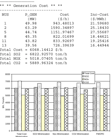
The comparison on the results with total cost minimization, SO2 minimization, NOx Minimization, CO2 minimization, and the proposed FMOPF is shown in Fig.3.

(10)

5

6161.4 $/h and 6104.2 ton/h, respectively and the

minimum CO2 solution results in the highest NOX emission of 5187.67 ton/h.

In contrast, the proposed FMOPF is effectively trades off all objectives in the fuzzy reasoning sense leading to the most compromise solution. Note the FMOPF results in the degree of satisfaction (

µ

'

) of 0.881.

Table 6. Dispatch results of minimum CO2 emission

condition

[image:10.595.72.303.354.636.2]

Table 7. Dispatch results of the proposed FMOPF

---

** ** Generation Cost ** ** ---

0 1000 2000 3000 4000 5000 6000 7000 8000 Total Cost Minimization

SO2 Minimization Nox Minimization CO2 Minimization FMOPD

$ /h , T o n s /H Total Cost SO2 NOx CO2

Fig. 3. The comparison on the results with different objective functions.

5. CONCLUSIONS

In this paper, a fuzzy multi-objective optimal real power flow (FMOPF) with transmission line limit and transformer loading constraints is successfully trading off between the total system operating cost, SO2

emission, NOx emission, and CO2 emission, satisfying

transmission line limits and transformer loading constraints. The proposed FMOPF results in a

compromise solution and can potentially be applied to overcome the difficulties of obtaining the weight or equivalent cost of emission.

ACKNOWLEDGMENT

This work was supported by Sripatum University.

NOMENCLATURE Known Variables x NO EC , x SO

EC , and

2

CO

EC : the total system NOx , SOx,

and CO2 emissions, respectively (ton/h),

) ( Gi NO P E

x , ESOx(PGi), and ECO2(PGi): the NOx, SO2, and

CO2 emissions of the generator connected to bus i,

respectively (ton/h), )

(PGi

F : the operating cost of the generator connected to bus i ($/h),

BG : set of buses connected with generators

max

l

f : MVA flow limit of line or transformer l (MVA)

NB : total number of buses

NT : total number of on load tap-changing transformers

Di

P : total real power demand at bus i (MW)

max

Gij

P : real power generation of the linearized cost

function segment j of generator at bus i (MW)

max

Gij

P : maximum real power generation of the linearized

cost function segment j of generator at bus i (MW)

max

Gi

P : maximum real power generation at bus i (MW)

min

Gi

P : minimum real power generation at bus i (MW)

Di

Q : reactive power demand at bus i (MVAR)

max Gi

Q : maximum reactive power generation at bus i

(MW)

min

Gi

Q : minimum reactive power generation at bus i

(MW)

inc Gi

R : ramping rate limit of generator i when increasing

real power generation (MW/min)

dec Gi

R : ramping rate limit of generator i when decreasing

real power generation (MW/min)

Min : time interval in minute (min)

ij

S : linearized incremental cost segment j of

generator at bus i ($/MWh)

max

i

T : maximum tap setting of transformer i (MW)

min

i

T : minimum tap setting of transformer i (MW)

max

i

V : maximum voltage magnitude at bus i (kV)

min

i

V : minimum voltage magnitude at bus i (kV)

ij

y : magnitude of the y_ij element of Ybus (mho)

ij

θ

: angle of the y_ij element of Ybus (radian)

Unknown Control Variables

Gi

(11)

6

connected to bus i (MW),

i

T : tap setting of transformer i (MW)

i

V : generator voltage magnitude at bus i, i∈BG

(kV)

State and Output Variables

FC : total system fuel cost ($/h)

l

f : MVA flow of line or transformer l (MVA)

NC : total number of line flow and transformer

loading constraints

NR

: total number of generator ramprate constraints

NV

: total number of bus voltage magnitude constraints

i

P : injection real power at bus i (MW)

loss

P : total system real power loss (MW)

Gi

Q : reactive power generation at bus i (MVAR)

i

V : voltage magnitude at load bus i, i∉BG (kV)

ij

δ

: voltage angle difference between bus i and j

(radian)

REFERENCES

[1] Yong-Lin Hu and William G. Wee. 1994. A Hierarchical System for Economic Dispatch with Environmental Constrains. IEEE Trans. Power Syst.,

9(2): 1076-1082.

[2] R. Ramanathan. 1994. Emission Constrained Economic Dispatch. IEEE Trans. Power Syst., 9(4):

1994-2000.

[3] Chao-Ming Huang, H. T. Yang, and C. L. Huang. 1997. Bi-Objective Power Dispatch Using Fuzzy Staisfaction-Maximizing Decision Approach. IEEE Trans. Power Syst., 12(4): 1715-1721.

[4] Victoria L. Vickers, Walter J.Hobbbs, Suri Vemuri and Daniel L.Todd. 1994. Fuel Resource Scheduling With Emission Constraints. IEEE Trans. Power Syst., 9(3): 1531-1538.

[5] Chao-Ming Huang and Yann-Chang Huang. 2003. A Novel Approach to Real-Time Economic Emission Power Dispatch. IEEE Trans. Power Syst., 18(1):

288-294.

[6] J. H. Talaq, Ferial and M.E. El-Hawary. 2003. Minimum Emission power Flow. IEEE Trans. Power Syst., 9(1): 429-435.

[7] P. Venkatesh, R. Gnanadass and Narayana Prasad Padhy. 2003. Comparison and Application of Evolutionary Programming Techniques to Combined Economic Emission Dispatch with Line Flow Constraints. IEEE Trans. Power Syst., 18(2):

688-697.

[8] H. J. Zimmermann. 1987. Fuzzy Sets, Decision Making, and Expert Systems. Boston: Kluwer

Academic Publishers,

(12)

K. Krajangpan, B. Neammanee and S. Sirisumrannukul / GMSARN International Journal 2 (2008) 7 - 14

7

Abstract— The key issue of wind energy conversion systems is how to efficiently operate the wind turbines. This issue

relies on the location where the turbines are operated. In addition, the control system with respect to machine operation and power production is essential in order to extract power from the turbines as much as possible regardless of wind

speed.The control performance of a MPPT controller with a grid connected wind turbine is therefore proposed in this

paper with two objectives.The first objective is to maximize the output power from the wind turbine by the maximum

peak power tracking (MPPT) method.The second objective focuses on the output power from a DC generator directly

coupled to the grid via a DC/AC converter or line side converter. Experiments are conducted with a 7.5kW grid

connected system, using step wind speeds and a real wind speed data set from a site in a southern province of Thailand

as the input of a wind simulator. The experimental results can confirm good MPPT performance and low harmonic

distortion in the grid connected line side converter.

Keywords— Maximum peak power tracking, MPPT, wind energy conversion, grid connected.

1. INTRODUCTION

As the impact of climate change has become public concern and the security of energy procurement is an issue, wind has become one of the fastest growing energy sources and is expected to continue growing in the electricity supply industry. The key issue of wind energy conversion systems is how to efficiently operate the wind turbines. This issue relies on the location where the turbines are operated. That is, the wind turbines should be placed where wind speed is strong and reasonably constant. In addition, the control system with respect to machine operation and power production is essential in order to extract power from the turbines as much as possible.

In general, a wind turbine is mechanically designed to produce its rating at a certain wind speed which is referred as rated wind speed. For wind speeds below the rated one, the main task of a controller is to capture the maximum power output. This task can be achieved by the maximum peak power tracking (MPPT) method.

References [1-3] propose a MPPT technique to track the maximum peak power without wind turbine characteristics. However, types of load are not considered. References [4, 5] implement controllers for grid connection via a line side converter and a transformer. The result is impressive in that active and reactive power can be directly and separately controlled with power factor near unity but the DC input source is not taken into account. It is therefore proposed in this paper a MPPT-based technique with consideration of

K. Krajangpan, B. Neammanee (corresponding author) and S. Sirisumrannukul are with Department of Electrical Engineering, King Mongkut's Institute of Technology North Bangkok 1518 Bangsue, Bangkok 10800, Thailand. Phone: (+66)2913-2500-24 Ext: 8420; Fax:

(+66)2585-7350; E-mail: bln@kmutnb.ac.th.

grid connection. The developed controller has two main objectives. [9-10]

The first objective is to maximize the output power from a wind turbine by the MPPT method. The second objective focuses on the output power from a DC generator coupled with a boost type converter to increase the DC bus voltage and directly coupled to the grid via a DC/AC converter or line side converter. Experiments are conducted with a 7.5kW grid connected system, using step wind speeds, variable wind speeds and a real wind speed data set from a site in a southern province of Thailand as the input of a wind simulator.

2. SYSTEM DESCRIPTION

A MPPT controller with a grid connected wind turbine is shown in Fig. 1. The system composed of three parts. The first part is the wind turbine coupled with a gear box and a DC generator. The wind turbine captures the energy from the wind and increases speed by the gear box to match speed of the generator. The second part is the MPPT controller composed of a power unit and control unit. The power unit consists of a boost converter which has two main functions. The first function is to amplify the DC link voltage to obtain enough voltage to match that of a 7.5 kW line side converter. The second function is to control the DC-bus output voltage for power flow control from the wind turbine to the grid to obtain the maximum peak power. The last part is a 7.5kW line side converter working as the front end of this system. The main function of the line side converter is to flow the energy production from the system to the three phase grid with a power factor of near unity. The lower part of the figure is a control unit consisting of the developed the MPPT controller, a data acquisition system and a line side converter controller. The MPPT controller receives the rotational speed form a rotary encoder, currents and voltages. The MPPT then builds a control command and sends it to the boost converter. K. Krajangpan, B. Neammanee and S. Sirisumrannukul

(13)

8

Fig. 1. MPPT controller with grid connected system for wind turbine.

2.1 Wind Turbine Characteristics

In order to describe wind turbine control schemes, a brief review of wind turbine characteristics is given here. The wind turbine characteristics are generally governed by (1) to (5).

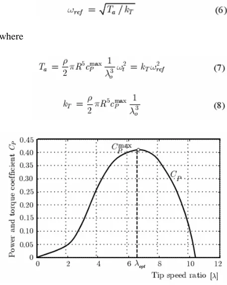
Equation (3) reveals that the power coefficient CP is a function of tip-speed ratio λ, which is defined by Equation (5). The CP - λ relationship is graphically

shown in Fig. 2. This figure is obtained from a real 3 kW horizontal axis wind turbine. The goal of control schemes for maximum wind power extraction is to keep wind turbine operating at their optimal tip-speed ratio, where the maximum energy conversion efficiency of

wind turbine can be reached. In Figure 3, C_Pmax is 0.4. In

order to simplify the following discussion,the parameter ηin (4) is assumed to be unity. Therefore, P_e is equal to

out P .

The power coefficient characteristic of a wind turbine has a single maximum at a specific value of the tip speed ratio. When the rotor operates at constant speed, the power coefficient will be maximum at only one wind speed. To achieve the highest annual energy capture, the value of the power coefficient must be maintained at the maximum level all the time, regardless of the wind speed [4]. For this reason, maximizing energy capture is to keep operating points at (λ0,cPmax) of Fig. 2.

Figure 3 shows a power-rotational speed curve with seven different wind speeds (υ1,υ2, ...,υ7). Path A-B in

the figure represents the optimum tracking path on which

each operating point has max P

C to build a rotational speed reference command, ωref, for the controller.

where

Fig. 2. Power coefficient CP(λλλλ) of real 3 kW wind turbine.

Fig. 3. Power characteristic and optimum power tracking paths.

2.2 Maximum Peak Power Tracking

Figure 4 shows typical characteristics of power and torque versus tip speed ratio of a wind turbine that needs to be controlled. The main purpose of the MPPT

controller is to maintain the operating point at max

m

P for

any wind speeds in the below rated wind speed region. At any instant of time, the operating point can be at the positive slope of the curve Fig.4 (the left hand side of the

max

m

[image:13.595.295.523.108.394.2]

(14)

9

maximum. This can be achieved by decreasing load

current, which results in an increase in rotational speed. Conversely, if the operating point lies on the right hand side of the peak, the load current has to be increased, resulting in a decrease in the rotational speed.

Fig. 4. MPPT process.

2.3 Line Side Converter

The line side converter links the MPPT unit with the grid. Figure 5 shows the three phase line side converter (power unit) that converts AC voltage to DC voltage by a space vector PWM converter. The per phase voltage equation can be written as in (9)-(11). [4-8]

Fig. 5. Line side converter (power unit).

Transforming (9)-(11) in three phases in stationary reference frame to two phase synchronous reference frame (d-, q-axis) gives:

For the balance three phase system,

The converter power, Pconv, and current, iconv, can be calculated by (15) and (16) [3].

The capacitor current, Icap, and DC bus voltage, Vdc,

can be calculated by (17) and (18).

With the transformation of (12)-(18) into s-domain, a block diagram in d-, q-axis reference frame can be constructed as shown in the right hand side of Fig. 6 (rectifying model). It is clear that there is voltage cross coupling between v_dn and vqn. To have independent

control of Vdc, the coupling voltage should be

[image:14.595.73.303.418.624.2]

compensated by a controller [4-5].

Fig. 6. Line side converter with voltage decoupling control.

3. CONTROL BLOCK DIAGRAM

3.1 MPPT Controller with Grid Connected Wind Turbine

Figure 7 shows the power circuit connection of this system composed of the MPPT controller with the boost converter, the line side converter and the grid. The MPPT controller receives the rotational speed, w ,

generator voltage, V , and current, g i , to calculate a g

change of rotational speed to obtain the maximum output power. The MPPT controller increase or decrease the speed by decreasing or increasing the duty cycle of the full-bridge converter. Accordingly, the output voltage will decrease/increase. The voltage will be stepped up by the transformer T1 and rectified by the full bridge and

the capacitor C1 in order to match the voltage of the line

(15)

10

3.2 MPPT Controller

The MPPT controller in the lower left corner of Fig. 7 can be explained in more detail as shown in the block diagram in Fig. 8. The top part of the diagram which is enclosed in the dotted line represents the MPPT controller built from (19) and (20). The MPPT controller receives the generator current, voltage and rotational speed from the plant as inputs and uses them to calculate the slope of the power-speed curve. The rate of change of power is compared with the reference (zero rate of change of power). The error is multiplied by the dc gain,M , to generate the current reference for the PI controller of the plant control system.

The tracking process can be achieved by decreasing load current, which results in an increase in the rotational speed. On the other hand, if the operating point lies at the right hand side of the peak power point, the load current has to be increased, resulting in the decrease in the rotational speed. The step increase or decrease of load current is made with reference to the relative position with P_mmax. This tracking methodology is called the perturbation and observation method (P&O). The current reference is calculated from

The slope of instantaneous power curve is given by

The current reference is updated by the MPPT controller at every time step Ts. The above mentioned

actions bring the operating point towards Pmmax by step-by-step increasing or decreasing the rotational speed.

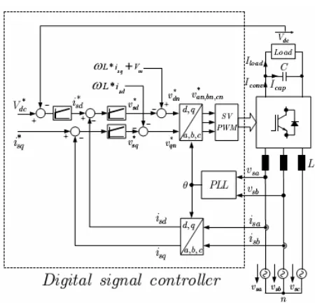
3.1 Line Side Converter Controller

In Fig. 6, the voltage cross coupling is compensated by feeding isd and isq with gain wL on the left hand side of

Fig.6. After the voltage is decoupled, the DC bus voltage

is controlled by two loops: current and voltage loops. The current isq does not affect the bus voltage and

therefore it is not used and the value of isqis set to zero.

Fig. 8. Block diagram of the MPPT control system with grid connected wind turbine.

The line side converter controller in the lower right corner of Fig. 7 can be explained in more detail as shown in the block diagram of Fig. 9. The controller of the line side converter is controlled in the d-, q-axis reference frame. The transformation between three phases and the

d-, q-axis requires an angle of phase voltage. A phase locked loop (PLL) to calculate the angle of phase voltage, θ*, is shown in Fig. 4 [6]. The PLL is composed of voltage transformation, sine and cosine calculation and PI controller. The parameter θ* in the transformation is obtained by integrating frequency command ω*. If the frequency is identical to the grid frequency, the voltages

sd

v and vsq become DC values, depending on the angle

θ*_{. A PI regulator is used to obtain that value of}_ω*_,

which drives the feedback voltage vsq to the command

value * sq

v . The magnitude of the controlled quantity vsq

(16)

11

voltages and sin(θ*) or cos(θ*). This system sets *

0 sq

v = .

Fig. 9. Line side converter control block diagram.

4 CASE STUDY

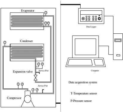
Test System

[image:16.595.73.298.94.310.2]

There are two main parts of the test system shown in Fig. 10: 1) a wind turbine simulator [11] on the left hand side of Fig. 10 and 2) a purposed wind turbine controller on the right side of Fig. 10. The data of the wind turbine is provided in appendix. The first part is given in detail in [11] and not repeated here because of limited space. The proposed controller consists of a boost converter connected between a generator line side converter and the grid (a load), voltage and current sensors, a data acquisition unit and a DSC controller. The controller board uses a high performance 16 bits dsPIC30f6010 combining the advantage of a high performance 16-bit microcontroller (MCU) and a high computation speed digital signal processors. Software was implemented in this DSC and performed to link a personal computer via two RS232 ports: one for transferring wind speed data to the DSC board and the other for sending parameters (e.g., Pe, i , g v , g w ) to the computer. g

Fig.10. The test system.

4.1 MPPT Control Trajectory with Step Wind Speed

The experiment began by starting up the wind turbine simulator at a wind speed of 4.5m/s to verify the tracking performance of the developed MPPT controller. The controller would try to track the maximum peak power as fast as possible by reducing P_e and thus resulting in an increase in w_t. When an operating point with the maximum power was found (i.e., dPt/dw =t 0), the controller tried to keep staying at that point.

The objective of this experiment was to track the maximum output power of the turbine. The wind simulator was started at a wind speed of 4m/s , stepped up to 4.5, 5 and 6 m/s respectively and run until steady state. The MPPT controller would capture maximum powers of 260, 420, 600 and 900 W respectively. The power versus rotational speed is shown in Fig. 11 and the output torque versus rotational speed is shown in Fig. 12. It is clearly seen that at the maximum output power, the aerodynamic torque are not maximum. Figure 13 (a) shows the relationship between cP and time obtained from the experiment. It can be seen from the figure that in this case, the MPPT controller can manage to keep c_P at 0.4 for the four step wind speeds. The power for each wind speed is shown in Figure 13 (b).

Fig. 11. The control trajectory of MPPT controller in the power versus rotational speed with various wind speed.

MPPT Control Trajectory with Real Wind Speed Data

This experiment used a real wind speed data set obtained from a site in Trung, a province situated in the southern part of Thailand, as the input of the wind turbine simulator. The data are classified as variable wind speed. Figure 14 shows the real wind speed data and the output power controlled by the MPPT controller. Figure 15 plots the control trajectory of the output power versus rotational speed. It is clear that the MPPT controller can track the maximum with the variable wind speed.

Grid Connect Converter

(17)

12

conventional PI controller is implemented. Figure 16 shows the dynamic performance of the line side converter, the DC link voltage and currents i_sd and i _sq

response for step load disturbance rejection. It can be seen that, the line side converter controller decrease isd to regulate the DC link voltage with low percentage of overshoot.

Fig. 12. The control trajectory of MPPT controller in the torque versus rotational speed with various wind speed.

Fig. 13. Output power and power coefficient with time.

Figure 17 shows the phase voltage and phase current of the grid connected line side converter. It can be seen that voltage and current are 180 degree out of phase. Therefore, the power flow from the wind turbine to grid with a phase current near sinusoidal with low harmonic distortion.

CONCLUSION

The control performance of the MPPT controller is verified by the developed 7.5 kW wind turbine simulator. The MPPT controller and line side converter are implemented on a dsPIC 30f6010 digital signal controller board with C language. Experiments are set up for testing the control performance of the MPPT controller and line side converter in inverting modes with grid connection. The experimental results confirm that the system can track the maximum output power with

various wind speeds and can regulate the DC bus voltage under nonlinear load generated from the wind turbine with nearly sinusoidal line side current, near-unity power factor and low harmonic distortion. The advantages of the MPPT controller are that it does not require any knowledge of a machine model, and turbine characteristic curves. The developed MPPT controller is useful in case of, for example, dirty blades, varying local air flow effects or blades with non-optimum pitch angles. Although these factors change the characteristics of the wind turbine, they do not affect the proposed control strategy.

Fig. 14. Real wind speed and the corresponded output power.

Fig. 15. The control trajectory of MPPT controller in the power versus rotational speed with various wind speed.

ACKNOWLEDGMENT

The authors would like to give a special thank to Department of Alternative Energy Development and Efficiency, Ministry of Energy, Thailand for the wind speed data used in the experiments.

(18)

13

Fig.16. DC bus voltage with step wind speed.

Fig. 17. Line voltage, vsa and current, isa in inverting

mode.

REFERENCES

[1] Neammanee, B., Chatratana, S. 2006. Maximum Peak Power Tracking Control for the new Small Twisted H-Rotor Wind Turbine. In Proc. of

International Conference on Energy for Sustainable Development: Issues and prospect for Asia, Phuket, Thailand, 1-3 Mar.

[2] Koutroulis E., Kalaitzakis K., Voulgaris N.C. 2001. Development of a Microcontroller-Based, Photo-voltaic Maximum power Point Tracking Control System. IEEE Trans. Power Electronics, 16: 46-54.

[3] Huynh, P., Cho, B.H. 1996. Design and analysis of a Microprocessor-Controlled Peak-power-Tracking System. IEEE Trans. Aerospace and Electronic

Systems, 32(1): 182 – 190.

[4] Sudmee, W., Neammanee, B. 2007. Control and Implementation of Line SideConverter for Doubly Fed Induction Generator of Wind Turbine.

International Conference on Electrical Engineering Electronics, Computer, Telecommunications and

Information Technology (ECTI), Chiang Rai,

Thailand, 9-12 May, 249-252.

[5] Dixon. J.W., Ooi. B.T. 1988. Indirect current control of a unity power factor sinusoidal boost type three-phase rectifier. IEEE Trans. Industrial Electronic, 35(4): 508-515.

[6] Rim, C.T., Choi, N.S., Cho G.C., Cho, G.H. 1994. A complete DC and AC Analysis of Three-phase Current PWM Rectifier Using d-q Transformation.

IEEE Trans. Power Electronics, 9(4): 390-396.

[7] Lee, D.-C. 2000. Advanced nonlinear control of three-phase PWM rectifiers. IEE Proc. on Electric

Power Appl., 147(5): 361-366.

[8] Kaura, V., Blasko, V. 1997. Operation of a Phase Locked Loop System under Distorted Utility Condition. IEEE Trans. Industry Application, 33(1): 58-63.

(19)

14

Renewable Energy Sources: A Survey. IEEE Trans.

Industry Electronics, 53(4): 1002-1016.

[10]Schulz, D., Fabis, R., Hanitsch, R.E. 2003. A Three Phase Power Electronic Converter for Grid Interration of Distributed Generation. Power Tech

Conference Proceedings, 23-26 June, Bologna,

Italy, 1002-1016.

[11]Neammanee, B., Sirisumrannukul, S., Chatratana, S. 2007. Development of a Wind Turbine Simulator for Wind Generator Testing. International Energy

Journal, 21-28.

APPENDIX

This is the wind turbine simulator parameters

Wind turbine type Horizontal

Number of blades 3 blades

Maximum power coefficient 0.40

Optimum tip speed ratio 5

Blade radius 2.25 m

Gear ratio 8

(20)

R. Eriksson and V. Knazkins / GMSARN International Journal 2 (2008) 15 - 20

15

Abstract— There are several possibilities to improve the small-signal stability in a power system. One adequate option

is to make use of available power system components that possess high controllability properties such as, for instance, high voltage direct current (HVDC) systems. This paper presents results from a study aimed at the investigation of small-signal stability enhancement achieved by proper coordinated control of multiple HVDC links. Modal analysis was used as the main tool for the theoretical investigation. The obtained results indicate that the coordinated control of several HVDC links in a power system may assist achieving in an essential increase of damping in the power system. Another important conclusion from the paper is that the possibilities of the coordination of the HVDCs to a certain extent depend on the structure of the grid, which can be investigated by examining the controllable subspace of the linearzied model of the power system.

Keywords— Coordinated control, HVDC, Modal analysis, Power System Stability.

1. INTRODUCTION

Modern interconnected electric power systems are characterized by large dimensions and high complexity of the structure and the dynamic phenomena associated with the power system operation and control. Power system deregulation that took place in many countries worldwide was one of the driving forces that stimulated a fuller utilization of power systems, which in some cases lead to a reduced stability margin, as the power systems became more stressed. Under these circumstances it becomes quite important to seek new possibilities of enhancement of both transient and small-signal stability of the power systems.

There are several obvious ways of improving power system stability, namely, (1) building new transmission lines, (2) installing new generation capacities, (3) better utilization of the existing equipment in the power system, or (4) a combination of the above. This paper is primarily concerned with third option, since compared to the other options it is less costly and can be easily implemented in a real power system. The central idea of the study presented in this paper is the utilization of several HVDC links for small-signal stability enhancement.

The central purpose of conventional HVDC transmission is to transfer a certain amount of electrical power from one node to another and to provide the fast controllability of real power transfer. If the HVDC link is operated in parallel with a critical ac line the load-flow of the ac line can be controlled directly. The presence of an HVDC can assist in improving the stability margin in the power system [1]. In case there are several HVDC

R. Eriksson (corresponding author) is with the Division of Electric Power Systems at Royal Institute of Technology, (KTH), Teknikringen

33, 100 44 Stockholm, Sweden. Email: robert.eriksson@ee.kth.se.

V. Knazkins is with the Division of Electric Power Systems at Royal Institute of Technology, (KTH), Teknikringen 33, 100 44

Stockholm, Sweden. Email: valerijs.knazkins@ee.kth.se.

links in the system, there is also a possibility of coordinating the HVDC links to enhance the operation of the system [by, for example, altering the load-flow patterns] and to improve the system stability evermore.

The power systems are known to be operated most of the time in the so-called `quasi-steady state'. That is to say, the power systems are always subject to various— often small—disturbances [2]. A change in the loading level or capacitor switching is typical examples of such small disturbances that sometimes give rise to oscillations in the power system. The oscillations are often positively damped and their magnitudes decrease after a while thus the system remains stable.

In case of negative damping of the oscillations the situation is opposite and may result in loss of synchronism unless preventive measures are taken.

2. CASE STUDY

The aim of this paper is to perform modal analysis using coordinated control of two conventional HVDC links in a benchmark power system. This paper also explores the possibilities brought by the controllability and coordination of the HVDC links to enhance the rotor angle stability upset by a disturbance.

In the benchmark power system, as is in all realistic cases, the turbine action is very slow compared to the fast controllability of the HVDC. The theory in this paper is based on small-signal analysis by linearizing the system around the stable or unstable equilibrium point. The modal analysis provides valuable information about the inherent dynamic characteristics of the system. By controlling the current through the HVDCs and using state feedback it is possible to move the eigenvalues to pre-specified locations in the complex plane and thereby increase the damping.

3. TEST POWER SYSTEM

The system in this case study consists of three generators connected to nodes A, B, and C. The HVDC links are Robert Eriksson and Valerijs Knazkins

(21)

R. Eriksson and V. Knazkins / GMSARN International Journal 2 (2008) 15 - 20

16

connected between nodes A and C and between B and C. The power production is large in node A and the load center is assumed to be in node C, i.e., there is a significant power flow from nodes A to C. The power can go either through the ac lines or through the HVDC links. An overview of the test power systems is shown in Fig. 1.

Fig. 1. Test Power system.

4. SYSTEM MODEL

The HVDC link is of a classical type, which implies that it consumes reactive power and that the active power can be controlled. The HVDC link consists of an ideal rectifier, inverter, and series reactor which models the dc-line and creates a smooth dc current. The power through the HVDC is controlled by controlling the firing angle, α. The firing angle is controlled by a basic PI-controller and the input is the set point current. The generators are modelled by the one axis model, described by equations (1)-(3) [3], thus three states per generator are used. The dynamics of the HVDC [4] are described in equations (4)-(16), where the subscripts “r” and “i” refer to rectifier and inverter, respectively.

δ ω&= (1)

(

)

1

m e

P P D

M

ω&= − − ω (2)

' '

' cos( )

' '

d d d

q f q

d d

x x x

E E E V

x x δ θ

 ₋ 

= − + − 

 

& (3)

where

δ is the rotor angle

ω is the rotor synchronous speed '

q

E∠δ, V∠θ are the voltage phasors at the internal and terminal buses

T

do' is the d-axis transient open-circuit time constant P_m is the mechanical power applied to the generator

shaft

D is the generator’s shaft damping constant

M is the machine inertia

x_d is the d-axis synchronous reactance

x

d' is the d-axis transient reactance E

f is the constant generator field voltage

1

( )

r i

d

d d d d

d d

R

I V V I

L L

= − −

& (4)

( )

setp

r I d d

x& =K I −I (5)

( )

setp

i I d d

x& =K I −I (6)

cos( ) ( )

setp

r xr KP Id Id

α = + − (7)

3 2 3

cos( )

r pu r

d r r C d

V V α X I

π π

= − (8)

3 2 _dc _dc pu dc

b b

r r d

b

V I

S V I

S

π

= − (9)

dc dc r dc

b b

r d d

b

V I

P V I

S

= − (10)

2 2 r r r

Q = − S −P (11)

cos( ) ( )

setp

i xi KP Id Id

γ = + − (12)

3 2 3

cos( )

i pu i

d i i C d

V V γ X I

π π

= − (13)

3 2 dc dc pu dc

b b

i i d

b

V I

S V I

S π = (14) dc dc i dc b b

i d d

b

V I

P V I

S

= (15)

2 2 i i i

Q = − S −P (16)

where

V

dr, Vdi are the per unit dc terminal voltages at the

rectifier and inverter

V

bdc, Ibdc, Sbdc are the base quantities at the dc

side for the voltage, current and power, respectively

X

cr, Xci are the unit commutation reactances R_d, L_d are the per unit dc line parameters

V

rpu, Vipu are the per unit ac bus voltages I

dsetp is the current set point through the HVDC

5. MODAL ANALYSIS

Pure Butane as refrigerant in domestic refrigerator freezer

Published by the

GREATER MEKONG SUBREGION ACADEMIC

AND RESEARCH NETWORK

c/o Asian Institute of Technology

P.O. Box 4, Klong Luang, Pathumthani 12120, Thailand

GMSARN

INTERNATIONAL JOURNAL

Vol. 1 No. 2

December 2007

ISSN 1905-9094

GMSARN

INTERNATIONAL JOURNAL

ADVISORY AND EDITORIAL BOARD

GMSARN MEMBERS

GMSARN

INTERNATIONAL JOURNAL

GREATER MEKONG SUBREGION ACADEMIC AND RESEARCH NETWORK

(http://www.gmsarn.org)

GMSARN International Journal

CONTENTS

1

2

∑

∑

∑

∑

∑

∑

3

{

µ

(

x

),

µ

(

x

),

µ

(

x

),

µ

(

x

)}

B

⋅

P

≤

d

~

µ

α

γ

µ

(x

)

µ

1

.

1

=

−

γ

α

µ

1

.

1

=

−

γ

α

µ

'

4

µ

5

_α

_α