Method of Successive Approximations for a Fluid Structure Interaction Problem

(1)

http://dx.doi.org/10.4236/am.2014.515223

Method of Successive Approximations

for a Fluid Structure Interaction

Problem

Aliou Gueye Sow, Ibrahima Mbaye

Department of Mathematics, University of Thies, Thies, Senegal Email: [email protected]

Received 17 May 2014; revised 25 June 2014; accepted 9 July 2014

This work is licensed under the Creative Commons Attribution International License (CC BY). http://creativecommons.org/licenses/by/4.0/

Abstract

In this paper, we present a method for solving coupled problem. This method is mainly based on the successive approximations method. The external force acting on the structure is replaced by

(

)

(

1, 1,

)

λ

= p x H+u x

λ

. Then we have a nonlinear equation of unknown

λ

to solve by successive approximations method. By this method, we obtain easily the analytic expression of the displace- ment. In addition, good results are obtained with only a few iterations.

Keywords

Beam Equation, Stokes Equation, Finite Elements Method, Successive Approximations Method

1. Introduction

Problem involved in fluid structure interactions occurs in a wide variety of engineering problem and therefore has attracted the interest of many investigations from different engineering disciplines. As a result, much effort has gone into the development of general computational method for fluid structure system by Osses, Fernandez, quarteroni, Blouza, Mbaye [1]-[7].

In this paper, successive approximations method is applied to solve a fluid-structure interaction problem. We replace the external force acting on the interface between fluid and structure by λ= p x H

(

₁, +u x

(

₁,λ

)

.

Then we introduce a nonlinear equation to solve by successive approximations such that the coupled problem is achievable.

By this method, we obtain good approximate solutions. In addition, the analytic solution of beam equation can be computed easily.

(2)

the one dimensional beam equation.

2. Presentation of the Problem

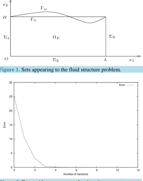
We denote by Ω_F the two dimensional domain occupied by the fluid, Γ_u the elastic interface between fluid and structure and Γ = ∑₁∑₂∑₃ be the remaining external boundaries of the fluid as depicted in Figure 1.

[ ] [

]

0

0,

L

0,

H

Ω =

×

defines the reference domain.

3. Governing Equations

3.1. Structure Equation

We start from the simple equation that governs the structure. The simplified beam equation is:

( )4

_{( )}

1 1 for 0 1

S

Du x = f x <x <L, (1)

( )

( )1

_{( )}

( )1

_{( )}

0 0 0

u =u L =u =u L = . (2)

where u is the displacement of the structure, fS is the external force of the structure,

3

12

Eh

D= , E is the

young modulus, h is the thickness of the structure This equation is good representation of the structure for small deformation.

3.2. Fluid Equation

We suppose that the fluid is governing by the Stokes equations for steady flow in Ω_F:

F

in

F

v p f

µ

− ∆ + ∇ = Ω , (3)

F

0 in

v

∇ ⋅ = Ω , (4)

1

on

v=g Σ , (5)

2

0 on

v n⋅ = Σ , (6)

1

2

0 on

v y ∂

= Σ

∂ , (7)

3

0 on

v pIn

n ∂

− + = Σ

∂ , (8) 0 on u

v= Γ , (9)

where v denotes the fluid velocity, p denotes the pressure, fF denotes the volume force of the fluid, µ the viscosity of the fluid and g denotes the inflow velocity profile of the fluid, n is the unit outward normal vector, I is the identity matrix, on the symmetric axis

Σ

₂ we have the non-penetration condition

2 0

v n⋅ =v = .

4. Formulation of Coupled Problem

The problem is to find u, v and p such that:

( )4

_{( )}

₍

_{( )}

₎

1 1, 1 for 0 1

Du x = p x H+u x <x <L (10)

( )

( )1

_{( )}

( )1

_{( )}

0 0 0

u =u L =u =u L = , (11)

F

in

F

v p f

µ

− ∆ + ∇ = Ω , (12)

F

0 in

v

∇ ⋅ = Ω , (13)

1

on

(3)

2

0 on

v n⋅ = Σ (15)

1

2

0 on

v y ∂

= Σ

∂ , (16)

3

0 on

v pIn

n ∂

− + = Σ

∂ , (17)

0 on u

v= Γ , (18)

We have a fluid structure interaction problem. The domain of the fluid depends on the displacement and the displacement depends on the velocity and the pressure of the fluid.

5. Successive Approximations Method

We assume that λ= p x H

(

₁, +u x

(

₁,λ

)

. Corresponding to each λ, we consider the coupled problem: ( )4

_{( )}

1 for 0 1

Du x =

λ

<x <L (19)

( ) ( )

( )1

_{( )}

( )1

_{( )}

0 0 0

u =u L =u =u L = , (20)

F

in

F

v

p

f

µ

− ∆ + ∇ =

Ω

, (21)

F

0 in

v

∇ ⋅ = Ω , (22)

1

on

v=g Σ , (23)

2

0 on

v n⋅ = Σ , (24)

1

2

0 on

v y ∂

= Σ

∂ , (25)

3

0 on

v pIn

n ∂

− + = Σ

∂ , (26) 0 on u

v= Γ , (27)

To solve this coupled problem, we need to solve a nonlinear equation of unknown λ define as:

(

)

(

1, 1,

)

p x H u x

λ

= +

λ

by the successive approximations method. Then we will find u, v and p.

Description of the Method

The weak formulation of the fluid and the structure is given by Grandmont, Murea [8] [9]. We summarize step by step our computational method to find

( )

λn such that:

0_{, the initial value is done}

λ ₍₂₈₎

(

)

(

)

1

1, 1,

n n

p x H u x

λ + ₌ ₊ λ _,₍₂₉₎  Step 1: We give λ0, the initial displacement and the fluid domain are compute.

 Step 2: We solve the Stokes equation by finite elements methods in the reference domain. We find

( ) (

v p

,

:

=

v p

0

,

0

)

,

 Step 3: we fine 1

(

0

)

1, 1, p x H u x

λ = + λ ,

 Step 4: Do: - λ0 =λ1,

- compute u x

(

₁,λ1

)

and Ω_F

( )

λ1 ,

- solve the stokes equation in

( )

1

F λ

Ω , we find

(4)

- we compute 1

(

0

)

1, 1,

p x H u x

λ = + λ ,

- While (

λ λ

1− 0 ≥tol),  Step 5: Give

λ

, u,

( )

v p

,

.

6. Numerical Results

For each

λ

, the analytic solution of the beam equations is

4 3 2 2

24 12 24

x Lx L x u

D

λ 

= _ − + _

 .

We assume that the velocity on Σ₁ is

v

= =

g

(

v v

₁

,

₂

)

such that v x x₁

(

₁, ₂

)

=30 1

(

−x₂2 H2

)

and

(

)

2 1

,

2

0 v x x

=

for all

(

x x

₁

,

₂

)

in Σ₁ Murea [10]. The parameter values of the fluid and the structure are:

Parameter related to fluid: The fluid velocity is µ =0.035 g cm s⋅ , the fluid density is

ρ

F =1 g cm3, the channel length is L=3 cm, the channel width H=0.5 cm _fF ₌

( )

0, 0 _.

Parameter related to structure: The structure thickness h=0.1 cm, Young’s modulus is

6 2

0.75 10 g cm s

E= × ⋅ , 4

10

tol= − .

We use the P b1 Lagrange finite element to approach the velocities and P1 Lagrange finite element is used to approach the pressure. FreeFem++ Hecht [11] is using for the numerical tests.

7. Conclusion

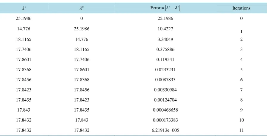
In this work, we applied successive approximations method to solve fluid structure interaction problem. This method gives good results when the displacement is small. After 11 iterations, we found a good approximate solution of the nonlinear equation and also we obtained the solution of coupled problem.

Table 1 and Figure 2 show that 1 0

Error= λ λ− decreases to zero when iterations increase. Figure 3 and Figure 4 display the behavior of the fluid flow and the pressure wave respectively after 11.

[image:4.595.197.430.424.718.2]

Figure 1. Sets appearing to the fluid structure problem.

(5)

Figure 3. Fluid velocity and structure displacement.

[image:5.595.90.539.242.471.2]

Figure 4. Fluid pressure.

Table 1. Different values of λ after 11 iterations.

1

λ λ0 1 0

Error=λ −λ Iterations

25.1986 0 25.1986 0

14.776 25.1986 10.4227

1

18.1165 14.776 3.34049 2

17.7406 18.1165 0.375886 3

17.8601 17.7406 0.119541 4

17.8368 17.8601 0.0233231 5

17.8456 17.8368 0.0087835 6

17.8423 17.8456 0.00330984 7

17.8435 17.8423 0.00124704 8

17.843 17.8435 0.000468658 9

17.8432 17.843 0.000173383 10

17.8432 17.8432 6.21913e−005 11

In a forthcoming work, we will be showed the theoretical convergence of λn+1 =p x H

(

₁, +u x

(

₁,λn

)

and also successive approximations method will be used to solve an unsteady fluid structure interaction problem.

References

[1] Osses, A. and Puel, J.P. (2000) Approximate Controllability for a Linear Model of Fluid Structure Interactiont. ESAIM

Control, Optimization and Calculus of Variation, 4, Article ID: 4976513.

[2] Fernandez, M.A. and Moubachir, M. (2003) And Exact Block Newton Algorithm for Solving Fluid Structure Interac- tion Problem. Compte rendu de l’académie des sciences, paris, Serie I, 336, 681-686.

[3] Fernandez, M.A. and Moubachir, M. (2005) A Newton Method Using Exact Jacobians for Solving Fluid-Structure Coupling. Computers and Structures, 83, 127-142.

[4] Quateroni, A., Tuveri, M. and Veneziani, A. (2000) Computational Vascular Fluid Dynamics, Problem Models and Methods. Computing and Visualization in Science, 2, 163-197. http://dx.doi.org/10.1007/s007910050039

[5] Blouza, A., Dumas, L. and Mbaye, I. (2008) Multiobjective Optimization of a Stent in a Fluid-Structure Context. Pro-

ceedingsof Genetic and Evolutionary Computation Conference (GECCO), 2056-2060.

http://dx.doi.org/10.1145/1388969.1389021

[6] Mbaye, I. (2012) Controllability Approach for a Fluid-Structure Interaction Problem. Applied Mathematics, 3, 213-216.

http://dx.doi.org/10.4236/am.2012.33034

[7] Mbaye, I. and Murea, C. (2008) Numerical Procedure with Analytic Derivative for Unsteady Fluid-Structure Interac- tion. Communications in Numerical Methods in Engineering, 24, 1257-1275.

(6)

stationnaire. Compte rendu de l’académie des sciences, Paris.

[9] Murea, C. and Maday, C. (1996) Existence of an Optimal Control for a Nonlinear Fluid Cable Interaction Problem. Rapport de Recherche CEMRACS, C.I.R.M., Luminy.

[10] Murea, C. (2005) The BFGS Algorithm for Nonlinear Least Squares Problem Arising from Blood Flow in Arteries.

Computers Mathematics with Applications, 49, 171-186. http://dx.doi.org/10.1016/j.camwa.2004.11.002

[11] Hecht, F. and Pironneau, O. (2003) A Finite Element Software for PDE FreeFem++.

(7)