Margin setting with high frequency data

Munich Personal RePEc Archive

Margin setting with high-frequency data

Cotter, John and Longin, Francois

2004

Online at

https://mpra.ub.uni-muenchen.de/3528/

Margin setting with high-frequency data

John Cotter

and François Longin

Abstract

Both in practice and in the academic literature, models for setting margin requirements

in futures markets classically use daily closing price changes. However, as well documented by

research on high-frequency data, financial markets have recently shown high intraday volatility,

which could bring more risk than expected. This paper tries to answer two questions relevant for

margin committees in practice: is it right to compute margin levels based on closing prices and

ignoring intraday dynamics? Is it justified to implement intraday margin calls? The paper

focuses on the impact of intraday dynamics of market prices on daily margin levels. Daily

margin levels are obtained in two ways: first, by using daily price changes defined with different

time-intervals (say from 3 pm to 3 pm on the following trading day instead of traditional closing

times); second, by using 5-minute and 1-hour price changes and scaling the results to one day.

Our empirical analysis uses the FTSE 100 futures contract traded on LIFFE.

Keywords: Clearinghouse, extreme value theory, futures markets, high-frequency data, intraday dynamics, margin requirements, risk management.

JEL Classification: G15

Version: 8.1 (July 27, 2006)

1

The authors would like to thank Lianne Arnold, Kevin Dowd, David Hsieh (the Editor), John Knight, Andrew Lamb, Alan Marcus, and Hassan Tehranian for their helpful comments on this paper. The first author acknowledges financial support from a Smurfit School of Business research grant. The second author acknowledges financial support from the ESSEC research fund.

2

Director of Centre for Financial Markets, Department of Banking and Finance, Smurfit School of Business, University College Dublin, Blackrock, Co. Dublin, Ireland, Tel.: +353-1-7168900. E-mail:

[email protected].

3

1. Introduction

The existence of margin requirements decreases the likelihood of customers' default,

brokers' bankruptcy and systemic instability of futures markets. Margin requirements act as

collateral that investors are required to pay to reduce default risk. 4 Margin committees face a

dilemma however in determining the magnitude of the margin requirement imposed on futures

traders. On the one hand, setting a high margin level reduces default risk. On the other hand, if

the margin level is set too high, then the futures contracts will be less attractive for investors due

to higher costs and decreased liquidity, and finally less profitable for the exchange itself. This

quandary has forced margin committees to impose investor deposits that represent a practical

compromise between meeting the objectives of adequate prudence and liquidity of the futures

contracts.

Let us describe as an example the way margins are set on the London International

Financial Futures and Options Exchange (LIFFE). For products traded on this exchange, margin

requirements are set by the London Clearing House (LCH) (for further details see London

Clearing House, 2002). The LCH risk committee is responsible for all decisions relating to

margin requirements for LIFFE contracts. Margin committees generally involve experienced

market participants who have widespread knowledge in dealing with margin setting and

implementation, through their exposure to various market conditions and their ability to respond

to changing environments (Brenner (1981)). The LCH risk committee is independent from the

commercial function of the Clearinghouse. In order to measure and manage risk, the LCH uses

the London Systematic Portfolio Analysis of Risk (SPAN) system, a specifically developed

variation of the SPAN system originally introduced by the Chicago Mercantile Exchange

margin requirements that are sufficient to cover potential default losses in all but the most

extreme circumstances.5 The inputs to the system are estimated margin requirements relying on

price movements that are not expected to be exceeded over a day or couple of days. These

estimated values are based on diverse criteria incorporating a focus on a contract’s price history,

its close-to-close price movements, its liquidity, its seasonality and forthcoming price sensitive

events. Market volatility is specially a key factor to set margin levels. Most important however

is the extent of the contract’s price movements with a policy for a minimum margin requirement

that covers three standard deviations of historic price volatility based on the higher of one-day or

two-day price movements over the previous 60-day trading period. This is akin to using the

Gaussian distribution where multiples of standard deviation cover certain price movements at

various probability levels.6

Clearinghouses are also beginning to recognize the importance of intraday dynamics. For

example, in 2002, the LCH has introduced an additional intraday margin requirement that is

initiated if price movements on a contract challenge the prevailing margin requirement (London

Clearing House, 2002). Specifically, an intraday margin requirement is initiated if a contract

price changes by 65% of the margin requirement originally set for that contract.7 In this case, the

4

Futures exchanges also use capital requirements and price limits to protect against investor default.

5

Alternative approaches in order to compute the margin requirement have been developed in the academic literature: Figlewski (1984), Gay et al (1986), Edwards and Neftci (1988), Warshawsky (1989), Hsieh (1993), Kofman (1993), Booth et al (1997), Longin (1999) and Cotter (2001) use different statistical distributions (Gaussian, historical or extreme value distribution) or processes (GARCH), Brennan (1986) proposes an economic model for broker cost minimization in which the margin is endogenously determined, and Craine (1992) and Day and Lewis (1999) model the distributions of the payoffs to futures traders and the potential losses to the futures clearinghouse in terms of the payoffs to barrier options.

6

For instance, under the hypothesis of normality for price movements, two standard deviations would cover 97.72% of price movements, and three standard deviations 99.87%.

7

Clearinghouse requires an additional margin payment for falling prices on a long position or for

rising prices on a short position. The possible impact of intraday price movements is now

clearly, and rightly so, of concern to risk management overseers for LIFFE contracts.

This paper tries to answer two questions relevant for margin committees in practice: is it

right to compute margin levels based on closing prices and ignoring intraday dynamics? Is it

justified to implement intraday margin calls? In order to answer these two questions this paper

takes into account the intraday dynamics of futures market prices in computing margin

requirements. All previous academic studies considered daily closing prices only, thus missing

potentially important information. In our study we obtain daily margin levels in two ways: first,

by using daily price changes defined with different time-intervals (say from 3 pm to 3 pm on the

following trading instead of traditional closing times); second, by using 5-minute and 1-hour

price changes and scaling the results to one day. The use of high frequency data may specially

be beneficial in order to get more precise estimates of risk measures as shown by Merton (1980).

The computation of risk management measures for futures at different frequencies has already

been considered by Hsieh (1993).8 Under the assumption of independence and identical

distribution (iid), daily margin levels obtained over different time-intervals should be on average

equal to and statistically different from daily margin levels obtained with closing prices.

Identically, scaled intraday margin levels estimated with 5-minute and 1-hour price changes

should be on average equal to daily margin levels obtained with closing prices. Any significant

differences may then be accounted for by the lack of iid behavior. In such a case, it may be

appropriate to set intraday margin levels in order to take into account specific intraday

8

dynamics. In our paper, different statistical distributions are also used to model futures price

changes: the Gaussian distribution, the extreme value distribution and the historical distribution.

A GARCH process is also used to take into account the time-varying property of financial data.

An application is given for the FTSE 100 futures contract traded on LIFFE.

The remainder of the paper is organized as follows. The statistical models used for the

distribution of futures contract price changes and the scaling methods are presented in the next

section. Section 3 provides a description of the FTSE 100 futures contract data used in the

application and a detailed statistical analysis of the intraday dynamics of the market prices.

Section 4 presents empirical results for margins by taking into account the intraday dynamics.

Finally, a summary of the results and some implications for decision makers are given in the

concluding section.

2. Statistical models and scaling methods

This section presents the different statistical models used to compute the margin level for

a given probability. We do not necessarily select the best model but rather consider distributions

that are used in practice by practitioners in charge of setting margins in derivative markets: the

Gaussian and historical distributions (commonly used), the extreme value distribution

(especially relevant for the problem of margin setting) and a GARCH type model (a conditional

distribution). Our main goal is to study the impact of intra-day dynamics in margin levels and to

show that such an impact is present whatever the distribution chosen. This section also presents

the scaling method (where available) to obtain daily margin levels from intraday price changes.

2.1 The Gaussian distribution

The Gaussian distribution is considered because it is a standard tool in risk management.

The unconditional Gaussian distribution of price changes requires the estimation of two

corresponds to the quantile where one is examining what margin requirement is sufficient to

exceed futures price changes over a time-period of length T for the probability level p. Denoted

by ML(p, T), the margin level is computed as follows :

(1) ML

(

)

( )

where N-1 is the inverse of the standardized Gaussian distribution.

As the expected price change can empirically be neglected over a short-time period (less

than one day in our study), the scaling law relating the margin ML(p, T) and the margin level for

a basic time unit (T=1) follows the T rule:

(2) ML p T( , )= T ML p⋅ ( ,1)

2.2 The extreme value distribution

One question that we may ask about the nature of risk management is whether the

clearinghouse should care more about ordinary market conditions or more about extraordinary

market conditions. In other financial institutions such as banks two distinct approaches are used:

value at risk models for ordinary market conditions and stress testing for extraordinary market

conditions (see Longin (2000)). The clearinghouse must also address both sets of market

conditions in margin setting so as to minimize the likelihood of investor default by examining a

range of probabilities of price movements associated with common and uncommon events. For

that reason the extreme value distribution is considered. It provides a precise model for the tail

of the distribution of price changes.9 Using the non-parametric estimation approach developed

by Hill (1975), the margin level ML(p, T) is computed as follows :

9

(3)

1

( , ) th n

ML p T r

N p

α

= ⋅

⋅

where rth is the tail threshold price change associated with the beginning of the sample of

tail observations, N the number of observations of price changes in the database, n is the number

of order statistics used to compute the tail parameter α. The tail parameter measures the degree

of tail thickness. It represents the number of bounded moments: moments lower than α are finite

and moments equal to and greater than α are infinite. Extreme value studies applied to financial

time-series (see Jansen and de Vries (1991) and Longin (1996) for example) have found tail

parameter estimates between 2 and 4 suggesting that not all moments of the price changes are

finite.

A result by Feller (1971) for the tail behavior under time-aggregation scales the results

by using a T1/α rule:

(4)

1

( , ) ( ,1)

ML p T ₌Tα_⋅ML p

Importantly the tail parameter α remains invariant to the aggregation process and also

has implications for empirical benefits in its actual estimation. Dacarogna et al (1995) have

shown that high-frequency tail estimation has efficiency benefits due to their fractal behavior. In

contrast, low frequency estimation suffers from negative sample size effects. Intuitively a large

(high) frequency data set has more observable extremes that a small (low) frequency one over

the same time interval thereby allowing for stronger inferences of these rare events. Furthermore

for ease of computation, the scaling procedure does not require further estimation, but only

involves parameters from the high-frequency analysis, shown to provide the most detailed

2.3 Historical distribution

The simplest way to calculate margins is as quantiles relying on the historical

distribution of returns. This is also the method with the least model risk. The historical

distribution provides margins representing a quantile using the full set of price changes ordered

in ascending fashion:

(5) ML p T( , ) min r_n, n 1 p N

= ≥ −

Note that there is no scaling law associated with the historical distribution and that we

are limited to in-sample margin estimation.

2.4 The GARCH process

All statistical models presented above are based on unconditional distributions and

cannot reflect current market conditions. As first noted by Hsieh (1991), modeling the

conditional heteroskedasticity is a key point in the margin setting context. As market conditions

may vary substantially over time, Hsieh suggests that the conditional density function may be

used in a dynamic margin setting process. In order to take into account current market

conditions a conditional process such as a GARCH process is used to address issues relating to

the dynamic features of futures contracts volatility (see Cotter (2001)).10 To model the

time-varying behavior of price changes suggested by the previous analysis, we use the GARCH

model developed by Bollerslev (1986) given by:

(6)

= =

− − +

+ =

p

i

q

j

j t j i

t i o

t

1 1

2 2 _βσ

ε α α

σ

10

for α₀,α_i,β_j≥0, α_i+β_j≤1.

The unconditional level of volatility is related to α0, persistence in volatility of the

innovations in ε_t2_−i given by αi and the persistence in past volatility σt2−j given by βj.

A single lag GARCH (1, 1) model is applied here to the price series at the end of the

sample during December 2000. Assuming the conditional distribution is Gaussian, results in

scaling using the T rule outlined earlier.

3. Data analysis

3.1 Data

The empirical analysis is based on transaction prices for the FTSE 100 futures contract

trading on the LIFFE exchange (data are obtained from Liffedata). This exchange has made a

clear distinction, between contracts that are either linked to an underlying asset or developed

formally on the basis of links to the recently developed European currency, the euro, and those

that remain linked to factors outside the currency area. The FTSE 100 represents the most

actively traded example of the latter asset type.

Data are available on the stock index contract for four specific delivery months per year,

March, June, September and December. Prices are chosen from those contracts with delivery

months on the basis of being the most actively traded using a volume crossover procedure. The

empirical analysis is completed for sampling frequencies of 5 minutes, 1 hour and 1 day. The

first interval is chosen so as to meet the objective of analyzing the highest frequency possible

and capturing the most accurate risk estimates but also avoids microstructure effects such as bid-

ask effects. For the daily frequency, the price changes are computed by taking different starting

(and ending) times to define the day: the beginning of the “day” can start from 9 am (the

daily price changes are then obtained. Log prices (or log prices to the nearest trade available) for

each interval are first differenced to obtain each period’s price change. The period of analysis is

for the year 2000 involving 247 full trading days corresponding to an average life span of an

exchange traded futures contract. The FTSE 100 futures daily interval encompasses 113

5-minute trading intervals and nine hourly trading intervals. A number of issues arise in the data

capture process. First, all holidays are removed. This entails New Year’s (2 days), Easter (2

days), May Day (1 day), spring holiday (1 day), summer holiday (1 day), and Christmas (2

days). In addition, trading took place over a half day during the days prior to the New Year and

Christmas holidays and these full day periods are removed from the analysis.

3.2 Basic statistics

Daily price changes defined with different time-intervals

In addition to examining daily price changes using closing prices that are the norm in

margin setting through the marking to market system, daily price changes can also be defined

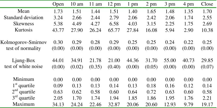
with different time-intervals. Basic statistics are reported in Table 1 and a time-series plot for

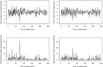
two of these time-intervals, using opening prices and closing prices are presented in Figure 1.

Whilst the mean price changes remain reasonably constant, other moments are more diverging

suggesting the dynamics for different intervals vary. For instance, skewness goes from 0.09 to

-0.47 and the kurtosis statistic goes from being platykurtic (-0.32) to leptokurtic (1.52). Also the

dispersion of various quantiles is considerable. Again dependency varies according to the

different time-intervals. Inferences for the squared price changes are similar although greater in

magnitude. However it can be observed that both time-series have similar time-varying features

evidencing volatility clustering with periods of high and low volatility but the diverging features

are clearly demonstrated as suggested by the magnitude of realizations. For example, the

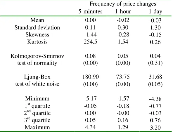
Price changes defined with different frequencies

Basic statistics are reported in Table 2 for price changes (Panel A) and for squared price

changes (Panel B) defined with different frequencies. We find different statistical behavior

according to the frequency of measurement with very strong dependency, excess kurtosis and

clear lack of normality recorded at the highest intraday level (5-minute intervals). To begin,

concentrating on the first four moments of the distribution, we find that kurtosis increases as the

frequency increases. For price changes, the (excess) kurtosis is equal to 0.26 for a 1-day

frequency, 1.54 for a 1-hour frequency and 254.50 for a 5-minute frequency. The high kurtosis

(greater than the value equal to 0 implied by normality) gives rise to the fat-tailed property of

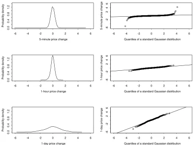
futures price changes. It is also illustrated by the probability density function and QQ plots of

the shapes of price changes for different frequencies given in Figure 2. The extent of fat-tails is

strongest for 5-minute realizations supporting the summary statistics and this would impact tail

quantiles (margins) for this frequency. Also, the magnitude of values for these realizations can

be very large as indicated by the scale of the density plots. These features generally result in the

formal rejection of a Gaussian distribution using the Kolmogorov-Smirnov test.11 Deviations

from normality are strongest at the highest frequency. The other moments emphasize the

magnitude and scale of the realizations sampled at different frequencies. On average, price

changes were negative during the year 2000 and unconditional volatility increases for interval

size. Selected quantiles reinforce divergences in magnitude at different frequencies. Similar

conclusions can be made for the proxy of volatility, the squared price changes, although the

skewness and kurtosis are more pronounced. Moreover, autocorrelation changes dramatically

according to frequency of estimation with much more dependency being recorded for 5-minute

price changes. For instance, the Ljung-Box test statistic is 180.90 for 5-minute price changes,

11

strongly rejecting the hypothesis of iid behavior, whereas in contrast this hypothesis is not

rejected at daily frequency (at 5% confidence level). This is also verified for squared price

changes.

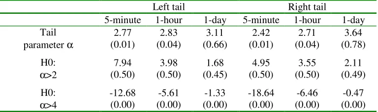
3.3 Extreme value analysis

Tail parameter estimates using different time-intervals to compute daily price changes

are presented in Table 3 for the left tail (Panel A) and the right tail (Panel B). Following

Huisman et al (2001) the point estimates are calculated using the weighted least squares

technique that minimizes the small-sample bias (see the appendix for details of the estimation

process). The point estimates range from 2.57 to 6.34 and the values are generally in line with

previous findings (see Cotter (2001)). As the tail parameter is positive, the extreme value

distribution is a Fréchet distribution that is obtained for a fat-tailed distribution of price changes.

The tail parameter is also estimated with higher frequency (Panel C). The tail parameter

value seems to be stable under the temporal aggregation. It tends to increase as we move to

higher frequency indicating a fatter tail recorded at intraday levels but this is not statistically

significant. As expected, the precision is also much improved by using 5-minute and 1-hour

price changes with lower standard errors. For example, for the left tail, the tail estimates with

standard error in parentheses are: 2.77 (0.01) for 5-minute intervals, 2.83 (0.04) for 1-hour

intervals and 3.11 (0.66) for daily intervals.

We also use the tail parameter estimates to test if the second and the fourth moment of

the distribution are well defined. For classical confidence level (say 5%), we are unable to reject

the hypothesis that the variance is infinite in any scenario, whereas we are able to reject the

3.4 Conditional estimation

Time-varying behavior is described from fitting the GARCH model to both intraday

price changes at 5-minute and 1-hour intervals and daily price changes from different

time-intervals at the end of December 2000.12 The GARCH estimates consistently indicate that the

conditional distributions exhibit persistence, with past volatility impacting on current volatility

as it is typical of GARCH modeling at daily intervals.13 Furthermore the conditional

distributions vary according to the time intervals analyzed that will give rise to different margin

requirements.

4. Model-based margin requirements

This section presents empirical results for margin requirements obtained with daily price

changes (4.1) and 5-minute and 1-hour price changes scaled to one day (4.2). In our analysis of

margin requirements we are interested in two separate questions: should margin requirements be

set with closing prices alone? Is there a justification for implementing intraday margin calls? We

now turn to these questions.

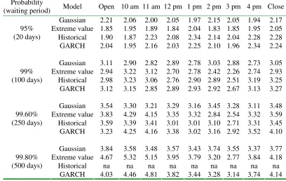
4.1 Margin requirement based on daily price changes

Table 4 presents margin requirements obtained with daily price changes for a long

position (Panel A) and for a short position (Panel B). Margin requirements are computed for a

given probability. Four different values are considered: 95%, 99%, 99.6% and 99.8%

12

Our application is given for illustrative purposes only. We could also have fit the GARCH model for full timeframe to obtain daily conditional margins throughout the year 2000.

13

corresponding to average waiting periods of 20, 100, 250 and 500 trading days.14 Thinking of

risk management for financial institutions, probabilities of 95% and 99% would be associated

with ordinary adverse market events modeled by value at risk models, and probabilities of

99.6% and 99.8% with extraordinary adverse market events considered in stress testing

programs. In the margin setting context, the probability reflects the degree of prudence of the

exchange: the higher the probability, the higher the margin level, the less risky the futures

contract for market participants, but the less attractive the contract for investors.

Margin requirements are computed with the statistical models previously presented:

three unconditional distributions (Gaussian, extreme value and historical) and a conditional

process (the GARCH process). For the presentation of the results, the extreme value distribution

will be the reference model as it presents many advantages (parametric distribution, limited

model risk, limited event risk) and as the problem of margin setting is mainly concerned with

extreme price changes. Beginning with the analysis of extreme value estimates, we first note

that variation occurs in the estimates based on the different time-intervals to define daily price

changes. For example, for a long position and a probability level of 95%, the estimated margin

level ranges from 1.83% to 2.05% of the nominal position. For the most conservative level of

99.8%, it ranges from 2.77% to 5.32%, almost double. Also there does not seem to be a

systematic pattern to these deviations. For instance, for a probability of 95%, the minimum is

obtained with 2 pm prices and the maximum for closing prices, and for a probability of 99.8%,

the minimum is obtained with 3 pm prices and the maximum for 10 am prices. The same

remarks apply to a short position. These findings suggest that the daily price change

14

distributions vary to some extent based on different time-intervals sampled suggesting separate

tail behavior for each price series.

Turning to the Gaussian estimates, some key insights are obtained. First, the measures

are almost identical for long and short positions due to the assumption of a symmetric

distribution of futures price changes and an average price change close to zero over the period

considered. In contrast, the extreme value distribution and the historical distribution take

account of the possibility of non-symmetric features in line with the oft cited stylized facts of

financial time series, and verified for the FTSE 100 futures contract of diverging upper and

lower distribution shapes. However, in line with all the estimates, diverging margin estimates

occur according to the time-intervals used to define price changes. For example, for a long

position and a probability of 95%, the estimated margin varies from 1.94% using 4 pm prices to

2.21% using opening prices. Traditional comparisons of extreme value and normal risk

estimates suggest the latter underestimates tail behavior due to its exponential tail decline that

results in relatively thin-tailed features. These findings hold for the FTSE 100 contract for high

probability levels of 99.6% and 99.8%. In contrast, for the relatively low probability level of

95%, this conclusion cannot be sustained and this is due to this confidence level representing a

common rather than extreme threshold. For instance, the probability of this event occurring

using daily data is once every 20 trading days representing a typical event rather than an

extreme one, although it is the latter events that need to be guarded against to avoid investor

default.

Then turning to the historical estimates, diverging margin requirements again occur

according to the time-interval chosen with the largest (smallest) estimate on a long position at

the 95% level happening at 1 pm (10 am). These estimates are based on using the historical

price series gathered for the year 2000. The historical estimates are confined to in-sample

using the historical distribution that tries to avoid investor default may not be able to model the

events that actually cause the default, whereas in contrast, extreme value theory specifically

models these tail values.

The margin requirements based on the unconditional distributions may be compared to

the conditional estimates using the GARCH process. Again it is clear that estimation at different

time-intervals necessitates diverging margins. For instance, the out-of-sample estimates

measured at 11 am (3 pm) represent the largest (smallest) possible margin requirements for a

long position. Comparing the extreme value and GARCH estimates provides information on the

distinction between unconditional and conditional environments facing margin setters. Distinct

patterns occur based on the volatility estimation for the last trading day of the sample

(December 29, 2000).

Thus this analysis suggests that Clearinghouses should consider setting margin

requirements based on different time-intervals so as to avoid ignoring intraday dynamics.

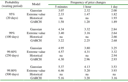
4.2 Daily margin requirement estimated with high-frequency price changes

Table 5 presents daily margin requirements obtained with 5-minute and 1-hour price

changes for a long position (Panel A) and for a short position (Panel B). Margin levels are

scaled to one day (see Section 2 for the presentation of the scaling method) and compared to the

ones obtained directly from daily price changes (average of daily margin levels obtained with

daily price changes defined on different time-interval as presented in Table 4). Different

statistical models are used: three unconditional distributions (the Gaussian distribution, the

extreme value distribution and the historical distribution) and a GARCH process. The historical

estimates are sometimes not available (na) due to the lack of a scaling formula or to data

The general conclusion that we can draw from the results presented in Table 5 is that

daily margin levels estimated with higher frequency (5-minute and 1-hour price changes) are

consistently higher than margin levels directly obtained from daily price changes. For the

Gaussian and the extreme value distributions, daily margin levels estimated with 5-minute price

changes are always higher than daily margin levels directly obtained with daily data. This is also

true for margin levels estimated with 1-hour price changes (except once at the 95% probability

level for the extreme value distribution). For example for Gaussian margins on a long position

the average scaled high-frequency margin levels are approximately 50% higher than daily

margin levels, which is significant from an economic point of view. A t-test also shows that this

difference is significant from a statistical point of view. Similar findings hold for the extreme

value distribution. The rationale for these results is as follows: the iid assumption of future price

changes, which is used for scaling margin levels computed with high-frequency data is not

verified in practice.

The Clearinghouse must address the implication of these findings. One way is to

introduce intraday margins that require additional payments from futures traders based on

intraday price movements. As we have seen, intraday price movements are not correctly

reflected in daily margins using scaling laws and this would encourage the Clearinghouse to

have an additional payments system for traders to protect against these (extreme) price

movements.

5. Summary and economic implications

This paper takes into account the intraday dynamics of futures prices changes in margin

setting. It then includes lost information that is unavailable with the traditional approach of

using closing prices in a marking to market system. The intraday futures price movements are

compute daily margin levels, and second high-frequency 5-minute and 1-hour price changes are

used to compute intraday margin levels that are then scaled to give daily margin levels.

This paper finds that intraday dynamics should be a key component in margin setting.

Daily price movements measured at different intervals can have a very tenuous relationship

suggesting that the common procedure of using only close of day prices neglects the dynamics

that investors actually face in trading futures. Daily margin levels estimated with high-frequency

data (5-minute and 1-hour price changes) are consistently higher than daily margin levels

directly obtained from daily price changes. Under the basic assumption of an iid process for

price changes, which is used for the scaling law, margin levels based on high-frequency data

should be more precisely estimated (it is the case) but on average not different from margin

levels directly obtained from daily price changes.

The two economic issues pointed out in the introduction of this paper were about the use

of closing prices to set daily margin levels and the justification of imposing intraday margins.

Let us consider first the issue of setting daily margins. A margin level computed with closing

prices may be substantially different from a margin level computed with another time-interval.

The same result is obtained with the scaled daily margins from high-frequency price changes,

which are substantially higher than the average margin level based on daily price changes. When

deciding about the daily margin level and taking into account the intraday dynamics of price

movements, the margin committee may consider margin levels computed with different

time-intervals. A conservative approach would lead to considering the highest margin level over all

time-intervals. The margin committee may also set daily margin level based on scaled margin

levels from high-frequency price changes. Note that the empirical study carried out in this paper

shows that both approaches (highest daily margin level based on price changes computed with

different time-intervals and scaled daily margin levels based on high-frequency price changes)

account the intraday dynamics in different but related ways. Let us consider now the issue of

intraday margins. This paper shows that if the margin committee set daily margin levels by

considering closing prices alone, it would to underestimate the margin level for a given level of

risk. Then it makes sense to add intraday margins in order to take into account the extra risk due

to the intraday dynamics. From a decision making point of view, the overall conclusion of this

paper is that by not accounting for intraday dynamics the Clearinghouse may set inadequate

Appendix

Estimation of the tail parameter

This appendix describes the estimation procedure for the tail parameter of the extreme

value distribution.

We use the method developed by Hill (1975) to estimate the tail parameter and also to

determine the distribution quantiles (margin levels). The Hill estimator is widely used in

empirical studies as it performs well for most time-series (Hall and Welsh (1984)) and is more

efficient than other estimators based on order statistics (Kearns and Pagan (1997)). It is used in

our scaling procedure for the extreme value method (Dacarogna et al, 1995)The Hill estimator

corresponds to the maximum likelihood estimator of the inverse of the tail parameter 1/α:

(A1)

(

)

1

1 1

ln ln

n

N i N n

i

r r

n

α = + − −

= −

De Haan et al (1994) shows that this tail estimator is asymptotically normal.

The issue in the estimation procedure is the choice of the optimal number of tail

observations (n) to include in the estimator (see Danielson et al (2001) for a discussion). The

dilemma faced is that there is a trade-off between the bias and variance of the estimator with the

bias decreasing and the variance increasing with the number of tail observations used. In order

to choose the optimal number of tail observations, we apply the regression method introduced

by Huisman et al (2001):

(A2) β β ε η

α( ) ( ), 1,....,

1

1

0+ + =

= n n n

For a weighted least squares regression of Hill estimates against associated numbers of tail

estimates that minimizes heteroskedasticity in the regression’s error term. Huisman et al. (2001)

find that the estimator works well from simulation of small samples (similar in size to that

References:

Bollerslev, T., Chou, R.Y. Kroner, K.F., 1992. ARCH Modeling in Finance: A Review of the Theory and Empirical Evidence, Journal of Econometrics, 52, 5-59.

Bollerslev T., Cai, J., Song, F.M., 2000. Intraday Periodicity, Long Memory Volatility, and Macroeconomic Announcement Effects in the US Treasury Bond Market, Journal of Empirical Finance, 7, 37-55.

Booth G.G., Broussard, J.P., Martikainen, T, Puttonen, V., 1997. Prudent Margin Levels in the Finnish Stock Index Market, Management Science, 43, 1177-1188.

Brennan, M.J., 1986. A Theory of Price Limits in Futures Markets, Journal of Financial Economics, 16, 213-233.

Brenner T.W., 1981. Margin Authority: No Reason for a Change, Journal of Futures Markets, 1, 487–490.

Cotter J., 2001. Margin Exceedances for European Stock Index Futures using Extreme Value Theory, Journal of Banking and Finance, 25, 1475-1502.

Cotter J., 2004. Minimum Capital Requirement Calculations for UK Futures, Journal of Futures Markets, 24, 193-220.

Craine R., 1992. Are Futures Margins Adequate ?, Working Paper, University of California – Berkley.

Dacarogna M.M., Pictet, O.V., Muller, U. A., de Vries, C.G., 1995. Extremal Forex Returns in Extremely Large Data Sets, Mimeo, Tinbergen Institute.

Danielson J., de Haan, L., Peng, L., de Vries, C.J., 2001. Using a Bootstrap Method to Choose the Sample Fraction in Tail Index Estimation, Journal of Multivariate Analysis, 76, 226-248.

Day T.E. Lewis, C.M., 1999. Margin Adequacy and Standards: An Analysis of the Crude Oil Futures Markets, Working Paper, Owen Graduate School of Management, Vanderbilt University.

Edwards F.R., Neftci, S.N., 1988. Extreme Price Movements and Margin Levels in Futures Markets, Journal of Futures Markets, 8, 639-655.

Feller W., 1971. An Introduction to Probability Theory and its Applications, John Wiley, New York.

Figlewski S., 1984. Margins and Market Integrity: Margin Setting for Stock Index Futures and Options, Journal of Futures Markets, 4, 385–416.

Gay G.D., Hunter, W.C., Kolb, R.W., 1986. A Comparative Analysis of Futures Contract Margins, Journal of Futures Markets, 6, 307–324.

De Haan L.S., Jansen, D.W., Koedijk, K., de Vries, C.G., 1994. Safety First Portfolio Selection, Extreme Value Theory and Long Run Asset Risks, in Galambos, C. (Ed.), Proceedings from a Conference on Extreme Value Theory and Applications. Kluwer Academic Publishing, Dordrecht, 471–487.

Hsieh D.A., 1991. Chaos and Nonlinear Dynamics: Application to Financial Markets, Journal of Finance, 46, 1839-1877.

Hsieh D.A., 1993. Implications of Nonlinear Dynamics for Financial Risk Management, Journal of Financial and Quantitative Analysis, 28, 41-64.

Huisman R., Koedijk, K., Kool, C.J.M., Palm, F., 2001. Tail Index Estimates in Small Samples, Journal of Business and Economic Statistics, 19, 208-215.

Jansen D.W., De Vries C.G., 1991. On the Frequency of Large Stock Returns: Putting Booms and Busts into Perspectives, Review of Economics and Statistics, 73, 18-24.

Kearns P., Pagan, A., 1997. Estimating the Density Tail Index for Financial Time Series, Review of Economics and Statistics, 79, 171-175.

Kofman P., 1993. Optimizing Futures Margins with Distribution Tails, Advances in Futures and Options Research, 6, 263–278.

London Clearing House, 2002, Market Protection, The role of LCH: regulatory framework, structure and governance, legal and contractual obligations, risk management, default rules, financial backing. London: LCH.

Longin F.M., 1996. The Asymptotic Distribution of Extreme Stock Market Returns, Journal of Business, 63, 383-408.

Longin F.M., 1999. Optimal Margin Levels in Futures Markets: Extreme Price Movements, Journal of Futures Markets, 19, 127-152.

Longin F.M., 2000. From Value at Risk to Stress Testing: The Extreme Value Approach, Journal of Banking and Finance, 24, 1097-1130.

Merton R.C., 1980. On Estimating the Expected Return on the Market, Journal of Financial Economics, 8, 323-361.

Figure 1. FTSE 100 futures contract daily price changes and squared price changes defined with opening and closing prices.

Time (in trading days)

P ri c e c h a n g e u s in g o p e n in g p ri c e s

0 50 100 150 200 250

-6 -4 -2 0 2 4 6

Time (in trading days)

P ri c e c h a n g e u s in g c lo s in g p ri c e s

0 50 100 150 200 250

-6 -4 -2 0 2 4 6

Time (in trading days)

S q u a re d p ri c e c h a n g e u s in g o p e n in g p ri c e s

0 50 100 150 200 250

0 1 0 2 0 3 0

Time (in trading days)

S q u a re d p ri c e c h a n g e u s in g c lo s in g p ri c e s

0 50 100 150 200 250

0 1 0 2 0 3 0

Figure 2. Probability density function and QQ plot for the FTSE 100 futures contract price changes defined with different frequencies.

5-minute price change

P ro b a b ili ty d e n s it y

-6 -4 -2 0 2 4 6

0 .0 0 .4 0 .8 1 .2

Quantiles of a standard Gaussian distribution

5 -m in u te p ri c e c h a n g e

-6 -4 -2 0 2 4 6

-6

-2

2

4

6

1-hour price change

P ro b a b ili ty d e n s it y

-6 -4 -2 0 2 4 6

0 .0 0 .4 0 .8 1 .2

Quantiles of a standard Gaussian distribution

1 -h o u r p ri c e c h a n g e

-6 -4 -2 0 2 4 6

-6

-2

2

4

6

1-day price change

P ro b a b ili ty d e n s it y

-6 -4 -2 0 2 4 6

0 .0 0 .4 0 .8 1 .2

Quantiles of a standard Gaussian distribution

1 -d a y p ri c e c h a n g e

-6 -4 -2 0 2 4 6

-6

-2

2

4

6

Table 1. Basic statistics for the FTSE 100 futures contract daily price changes defined with different time-intervals.

Panel A. Price changes

Open 10 am 11 am 12 pm 1 pm 2 pm 3 pm 4 pm Close Mean -0.04 -0.04 -0.03 -0.03 -0.03 -0.03 -0.04 -0.03 -0.03 Standard deviation 1.32 1.23 1.20 1.23 1.18 1.29 1.22 1.16 1.30

Skewness -0.13 -0.10 -0.30 -0.47 -0.32 -0.13 -0.14 -0.09 -0.15 Kurtosis 1.52 1.13 0.88 1.39 0.16 0.14 -0.05 -0.32 0.26

0.05 0.04 0.05 0.06 0.04 0.03 0.04 0.03 0.04 Kolmogorov-Smirnov

test of normality (0.10) (0.48) (0.11) (0.11) (0.46) (0.62) (0.57) (0.71) (0.31)

26.29 26.29 34.98 32.83 34.25 29.83 41.28 36.47 31.68 Ljung-Box

test of white noise (0.16) (0.16) (0.02) (0.04) (0.02) (0.07) (0.00) (0.01) (0.05)

Minimum -5.84 -4.92 -4.74 -5.73 -4.48 -4.54 -3.60 -3.13 -4.38 1st quartile -0.79 -0.86 -0.78 -0.76 -0.80 -0.79 -0.79 -0.80 -0.77 2nd quartile -0.04 -0.01 0.02 -0.01 0.03 -0.02 -0.04 0.02 0.00 3rd quartile 0.78 0.74 0.73 0.81 0.80 0.86 0.78 0.76 0.76 Maximum 4.26 4.06 3.59 3.09 2.59 3.20 3.02 2.48 3.20

Panel B. Squared price changes

Open 10 am 11 am 12 pm 1 pm 2 pm 3 pm 4 pm Close Mean 1.73 1.51 1.44 1.51 1.40 1.65 1.48 1.35 1.70 Standard deviation 3.24 2.66 2.44 2.79 2.06 2.42 2.06 1.74 2.55 Skewness 5.38 4.49 4.27 6.58 4.03 3.15 2.25 1.75 2.69 Kurtosis 43.77 27.90 26.24 65.77 27.84 16.08 5.94 2.90 10.38

0.30 0.29 0.28 0.29 0.25 0.25 0.24 0.22 0.25 Kolmogorov-Smirnov

test of normality (0.00) (0.00) (0.00) (0.00) (0.00) (0.00) (0.00) (0.00) (0.00)

44.01 34.91 21.78 21.00 44.36 31.70 55.00 40.73 29.85 Ljung-Box

test of white noise (0.00) (0.02) (0.35) (0.40) (0.00) (0.05) (0.00) (0.00) (0.07)

Minimum 0.00 0.00 0.00 0.00 0.00 0.00 0.00 0.00 0.00 1st quartile 0.09 0.13 0.13 0.14 0.13 0.18 0.16 0.12 0.14 2nd quartile 0.63 0.62 0.58 0.60 0.64 0.72 0.63 0.60 0.58 3rd quartile 2.05 1.70 1.74 1.94 1.85 1.86 1.95 1.76 2.21 Maximum 34.13 24.24 22.46 32.87 20.06 20.60 12.93 9.79 19.17

Table 2. Basic statistics for the FTSE 100 futures contract daily price changes defined with different frequencies.

Panel A. Price changes

Frequency of price changes 5-minutes 1-hour 1-day

Mean 0.00 -0.02 -0.03

Standard deviation 0.11 0.30 1.30

Skewness -1.44 -0.28 -0.15

Kurtosis 254.5 1.54 0.26

0.08 0.05 0.04

Kolmogorov-Smirnov

test of normality (0.00) (0.00) (0.31)

180.90 73.75 31.68 Ljung-Box

test of white noise (0.00) (0.00) (0.05)

Minimum -5.17 -1.57 -4.38

1st quartile -0.05 -0.18 -0.77 2nd quartile 0.00 -0.00 -0.03

3rd quartile 0.05 0.16 0.76

Maximum 4.34 1.29 3.20

Panel B. Squared price changes

Frequency of price changes 5-minutes 1-hour 1-day

Mean 0.01 0.09 1.70

Standard deviation 0.21 0.17 2.55

Skewness 107.99 5.24 2.69

Kurtosis 12 815.78 46.5 10.38

0.47 0.29 0.25

Kolmogorov-Smirnov

test of normality (0.00) (0.00) (0.00)

6 351.26 107.51 29.85 Ljung-Box

test of white noise (0.00) (0.00) (0.07)

Minimum 0.00 0.00 0.00

1st quartile 0.00 0.01 0.14

2nd quartile 0.00 0.03 0.65

3rd quartile 0.01 0.09 2.21

Maximum 26.73 2.46 19.17

Table 3. Tail parameter estimates and test of the existence of moments for the FTSE 100 futures contract price changes.

Panel A. Daily future price changes - Left tail

Open 10 am 11 am 12 pm 1 pm 2 pm 3 pm 4 pm Close

Tail parameter α

3.06 (0.65) 3.25 (0.69) 2.68 (0.57) 3.30 (0.70) 3.62 (0.77) 3.51 (0.75) 6.34 (1.35) 3.03 (0.65) 3.11 (0.66) H0: α>2 1.63 (0.45) 1.81 (0.46) 1.18 (0.38) 1.85 (0.47) 2.10 (0.48) 2.02 (0.48) 3.21 (0.50) 1.60 (0.45) 1.68 (0.45) H0: α>4 -1.43 (0.00) -1.08 (0.00) -2.32 (0.00) -0.99 (0.00) -0.49 (0.00) -0.65 (0.00) 1.73 (0.46) -1.50 (0.00) -1.33 (0.00)

Panel B. Daily future price changes - Right tail

Open 10 am 11 am 12 pm 1 pm 2 pm 3 pm 4 pm Close Tail

parameter α

2.58 (0.55) 3.63 (0.77) 4.34 (0.93) 3.77 (0.80) 4.20 (0.90) 3.48 (0.74) 4.96 (1.06) 4.08 (0.87) 3.64 (0.78) H0: α>2 1.05 (0.35) 2.11 (0.48) 2.53 (0.49) 2.20 (0.49) 2.46 (0.49) 2.00 (0.48) 2.80 (0.50) 2.39 (0.49) 2.11 (0.49) H0: α>4 -2.59 (0.00) -0.48 (0.00) 0.37 (0.14) -0.29 (0.00) 0.22 (0.09) -0.70 (0.00) 0.91 (0.32) 0.09 (0.04) -0.47 (0.00)

Panel C. High-frequency future price changes - Left and right tails

Left tail Right tail

5-minute 1-hour 1-day 5-minute 1-hour 1-day Tail

parameter α

2.77 (0.01) 2.83 (0.04) 3.11 (0.66) 2.42 (0.01) 2.71 (0.04) 3.64 (0.78) H0: α>2 7.94 (0.50) 3.98 (0.50) 1.68 (0.45) 4.95 (0.50) 3.55 (0.50) 2.11 (0.49) H0: α>4 -12.68 (0.00) -5.61 (0.00) -1.33 (0.00) -18.64 (0.00) -6.46 (0.00) -0.47 (0.00)

Note : this table gives the tail parameter estimates for the left tail (Panel A) and the right tail (Panel B) of the distribution of daily price changes and for the left and right tails (Panel C) of the distribution of 5-minute, 1-hour and daily price changes. It also provides a test of the existence of the moments of the distribution. The first line of the table gives the tail parameter estimate obtained with the method developed by Huisman et al (2001) with the standard error below in parentheses. The second and third lines give the results of a test of the existence of the second moment (the variance) and the fourth moment (the kurtosis) with the p-value below in parentheses. As the tail parameter corresponds to the highest moment defined for the distribution, the null hypotheses are defined as follows: H0: α > 2 and

Table 4. Margin levels based on daily price changes for the FTSE 100 futures contract.

Panel A. Long position

Probability

(waiting period) Model Open 10 am 11 am 12 pm 1 pm 2 pm 3 pm 4 pm Close Gaussian 2.21 2.06 2.00 2.05 1.97 2.15 2.05 1.94 2.17 Extreme value 1.85 1.95 1.89 1.84 2.04 1.83 1.85 1.95 2.05 Historical 1.90 1.87 2.23 2.08 2.34 2.14 2.04 2.28 2.28 95%

(20 days)

GARCH 2.04 1.95 2.16 2.03 2.25 2.10 1.96 2.34 2.24

Gaussian 3.11 2.90 2.82 2.89 2.78 3.03 2.88 2.73 3.05 Extreme value 2.94 3.22 3.12 2.70 2.78 2.42 2.26 2.74 2.93 Historical 2.98 3.23 3.06 2.76 2.90 2.89 2.51 3.19 3.25 99%

(100 days)

GARCH 3.12 3.15 2.85 2.89 2.93 2.92 2.67 3.13 3.27

Gaussian 3.54 3.30 3.21 3.29 3.16 3.45 3.28 3.11 3.48 Extreme value 3.83 4.29 4.15 3.35 3.32 2.84 2.54 3.32 3.59 Historical 3.59 3.39 3.41 3.01 3.01 3.10 2.71 3.31 3.45 99.60%

(250 days)

GARCH 3.23 4.25 4.16 3.38 3.02 3.16 2.92 3.52 4.10

Gaussian 3.84 3.58 3.48 3.57 3.43 3.74 3.55 3.37 3.77 Extreme value 4.67 5.32 5.15 3.95 3.79 3.20 2.77 3.84 4.18 Historical na na na na na na na na na 99.80%

(500 days)

GARCH 4.03 4.46 4.81 3.82 3.44 3.28 3.14 3.74 4.14

Panel B. Short position

Probability

(waiting period) Model Open 10 am 11 am 12 pm 1 pm 2 pm 3 pm 4 pm Close Gaussian 2.13 1.98 1.94 1.99 1.91 2.09 1.97 1.88 2.11 Extreme value 1.70 1.76 1.80 1.65 1.96 1.74 1.77 2.06 1.94 Historical 1.85 1.72 1.75 1.73 2.06 2.03 1.92 2.19 2.10 95%

(20 days)

GARCH 1.66 1.63 1.76 1.72 1.94 2.06 1.89 2.21 2.18

Gaussian 3.03 2.82 2.76 2.83 2.72 2.97 2.80 2.67 2.99 Extreme value 2.69 2.91 2.98 2.41 2.67 2.31 2.16 2.89 2.77 Historical 2.76 2.82 2.67 2.47 2.82 2.50 2.37 2.78 2.77 99%

(100 days)

GARCH 3.08 2.97 2.65 2.40 2.61 2.49 2.30 2.79 2.86

Gaussian 3.42 3.46 3.22 3.15 3.23 3.10 3.39 3.20 3.05 Extreme value 3.87 3.87 3.97 2.99 3.18 2.71 2.42 3.51 3.40 Historical 3.70 3.01 2.90 2.58 2.97 2.70 2.48 2.96 3.20 99.60%

(250 days)

GARCH 3.51 3.10 2.82 2.64 3.38 2.80 2.33 2.92 2.89

Gaussian 3.76 3.50 3.42 3.51 3.37 3.68 3.47 3.31 3.71 Extreme value 4.80 4.80 4.93 3.53 3.63 3.05 2.63 4.06 3.96 Historical na na na na na na na na na 99.80%

(500 days)

Table 5: Daily margin levels based on 5-minute, 1-hour and 1-day price changes for the FTSE 100 futures contract.

Panel A. Long position

Frequency of price changes Probability

(waiting period) Model _{5 minutes 1 hour 1 day}

Gaussian 3.07 2.52 2.07

Extreme value 2.17 1.64 1.92

Historical na na 1.75

95% (20 days)

GARCH 1.63 1.29 2.12

Gaussian 4.34 3.52 2.91

Extreme value 3.18 3.06 2.79

Historical na na 2.67

99% (100 days)

GARCH 3.32 2.65 2.99

Gaussian 4.95 4.00 3.31

Extreme value 4.48 4.12 3.47

Historical na na 2.90

99.60% (250 days)

GARCH 4.36 3.44 3.53

Gaussian 5.37 4.33 3.59

Extreme value 5.81 5.08 4.10

Historical na na na

99.80% (500 days)

GARCH 5.37 4.33 3.87

Panel B. Short position

Frequency of price changes Probability

(waiting period) Model _{5 minutes 1 hour 1 day}

Gaussian 3.07 2.32 2.00

Extreme value 2.33 1.47 1.82

Historical na na 1.93

95% (20 days)

GARCH 1.58 1.20 1.89

Gaussian 4.34 3.32 2.84

Extreme value 3.40 3.16 2.64

Historical na na 2.66

99% (100 days)

GARCH 3.22 2.25 2.68

Gaussian 4.95 3.80 3.25

Extreme value 4.57 4.31 3.32

Historical na na 2.94

99.60% (250 days)

GARCH 4.30 2.96 2.93

Gaussian 5.37 4.13 3.53

Extreme value 6.46 5.20 3.93

Historical na na na

99.80% (500 days)