A Novel Multi agent based PSO approaches for security Constrained Optimal Power Flows using smooth and non smooth cost functions

A Novel Multi agent based PSO approaches for security

Constrained Optimal Power Flows using smooth and

non-smooth cost functions

K. Ravi Kumar

Associate Professor EEE Department Vasavi College of Engineering,

Hyderabad

S. Anand

Senior Software Analyst Intergraph Consulting

Hyderabad

M. Sydulu

Professor ,EE Department National Institute of

Technology, Warangal

ABSTRACT

This paper puts forward two new evolutionary multi agent based particle swarm optimization algorithms for solving security constrained (line flows and bus voltages) optimal power flows. These two methods combine the multi agents in two dimensional and cubic lattice structures with particle swarm optimization (PSO). All agents occupy in a cubic and square lattice like environments, with agents fixed on a lattice point in the ascending order of their fitness values. To obtain the optimal solution, each agent in cubic and square lattice competes and cooperates with its neighbor. Making use of these agent-agent interactions, CLSMAPSO and TDLSMAPSO accomplish the purpose of minimizing the Fuel cost value while maintaining all the constraints. In this paper, a Variable constriction factor has been considered for TDLSMAPSO and CLSMAPSO. Both the smooth and non-smooth cost functions were considered to take the effect of multiple fuels and multiple valves effects in to consideration. The outcomes are compared with many other methods like Genetic Algorithms, Differential Evolution, Normal PSO and Ant Colony optimization etc., The OPF problem has been considered with three different cost functions to realize Optimal Power Flow using CLSMAPSO and TDLSMAPSO applied to IEEE 30 bus system. This unique method has the advantage of more agent interactions in case of CLSMAPSO which improved the convergence drastically compared to the Two dimensional structure used in paper by sivasubramani and Shanti swarup in reference[2]. It is found that the proposed method is found to be computationally fast, robust, superior and promising from its convergence characteristics.

General Terms

Newton-Raphson(NR) algorithm, Lattice, Agent, Smooth and Non-smooth cost functions.

Keywords

Multi agent systems, Optimization techniques, Particle swarm optimization, Optimal power flows, security constraints.

1.

INTRODUCTION

Optimal Power Flows was first setup in the early 1960‟s by Carpentier1 as an extension of conventional economic dispatch. Nowadays, utilities are facing rapid growth in the Electricity demand with slow fortification projects due to financial and political issues. Proper operation and planning requires consideration of different factors such as reduction of generation cost, losses, pollution, security of power system, and FACTS allocation etc…. In this regard Optimal power Flows (OPF) have been widely used in planning and real time operation of power systems for Reactive and active power

dispatch to minimize generation costs and system losses and to improve profiles of the voltages. The OPF generally meant to optimize set of objectives under set of constraints under consideration.

A vast variety of optimization techniques have been applied in solving the OPF problem such as non-linear programming, Quadratic Programming, Linear Programming, Newton based methods, Sequential unconstrained minimization technique, interior point methods, Genetic Algorithm, Evolutionary Programming. Heuristic algorithms such as Genetic Algorithms (GA) and Evolutionary programming which have been reported as show promising results for further research in this direction.

Recently, a new novel evolutionary computation technique, called Multi agent based Particle Swarm Optimization (MAPSO)2, has been proposed. Particle Swarm Optimization (PSO) is one of the evolutionary computation techniques. In PSO, search for an optimal solution is conducted using a population of particles, each of which represents a candidate solution to the optimization problem. It was developed through the simulation of flock of birds to search for food in an optimal manner through their velocity and position up gradation. The PSO technique has been widely used for the solving the optimization of various power system problems. However, the major drawback with PSO is that, it may need several iterations and may get trapped in local optima. Therefore, several strategies have been developed to overcome the limitations of PSO, such as modified PSO, and attractive and Repulsive PSO. These all were proved to be effective and boosted the development of MAPSO.

TDLSMAPSO and CLSMAPSO for OPF is discussed in section 5. The simulation results with different methods comparison are discussed in section 6. Finally, brief conclusions are deduced in section 7. References were given in section 8 and biographies were given in section 9.

2.

PROBLEM FORMULATION

OPTIMAL POWER FLOW

All The OPF problem is a static constrained non-linear optimization problem, the solution of which determines the optimal settings of control variables in a power system network satisfying different constraints. Hence, the problem is to obtain the solution for a set of non-linear equations describing the optimal solution of power system. It is expressed as

Min F(x,u) (1) Subject to g(x, u)=0

h(x, u)≤0

The objective function F is fuel cost of thermal generating units of the test system. g(x,u) is a set of non-linear equality constraints to represent power flow and h(x,u) is a set of non-linear inequality constraints(i.e., bus voltage limits, line MVA limits etc..). Vector x consists of dependent variables and u consists of control variables.

In most of the non-linear optimization problems, the constraints are being handled by generalizing the objective function using penalty terms. In this OPF problem, slack bus power PG1, bus voltages VL and line flows Ij are constrained

by adding them as penalty terms to objective function. Hence, the problem is generalized and can be written as follows.

𝐹𝑇∗= 𝐹𝑇+ 𝜆 𝐼𝑖− 𝐼𝑚𝑎𝑥 2+ (𝑃𝐺1− 𝑃𝐺1𝑙𝑖𝑚)2 𝑖∈𝑁𝐿

+ (𝑉𝑖− 𝑉𝑖𝑙𝑖𝑚)2 𝑖𝜖𝑁𝑃𝑄

+ 𝑄𝐺𝑖− 𝑄𝐺𝑖𝑙𝑖𝑚 2

𝑖𝜖𝑁𝑃𝑉

+ (𝑙𝑜𝑠𝑠𝑖)2 𝑖𝜖𝑁𝑙𝑖𝑛𝑒

2

Where 𝜆, the penalty factor, is given as

𝜆 = 𝑐𝑖

𝑁𝑢𝑚𝑏𝑒𝑟 𝑜𝑓 𝑔𝑒𝑛𝑒𝑟𝑎𝑡𝑜𝑟 𝑏𝑢𝑠𝑒𝑠 𝑉𝑖𝑙𝑖𝑚 and 𝑃𝐺1𝑙𝑖𝑚 are defined as

𝑉𝑖𝑙𝑖𝑚 =

𝑉𝑖𝑚𝑎𝑥 ; Vi> 𝑉𝑖𝑚𝑎𝑥

𝑉𝑖𝑚𝑖𝑛 ; Vi< 𝑉𝑖𝑚𝑖𝑛 (3)

𝑃𝐺1𝑙𝑖𝑚 =

𝑃𝐺1𝑚𝑎𝑥 ; PG1> 𝑃𝐺1𝑚𝑎𝑥

𝑃𝐺1𝑚𝑖𝑛 ; PG1< 𝑃𝐺1𝑚𝑖𝑛 (4)

3.

DIFFERENT COST FUNCTIONS

3.1

OPF Problem With Smooth Cost

Function

The OPF problem is to find the optimal combination of power generations that minimizes the total generation cost while satisfying an equality constraint and inequality constraints. The most simplified cost function of each generator can be represented as a quadratic function as given in eq (5) whose solution can be obtained by the conventional mathematical methods

FT = 𝑖∈𝑁𝐺(𝑎𝑖𝑃𝐺𝑖2 + 𝑏𝑖 𝑃𝐺𝑖+ 𝐶𝑖) (5)

While minimizing the total generation cost, the total generation should be equal to the total system demand plus the transmission network loss.

3.2

OPF Problem with Non-smooth Cost

Functions

In reality, the objective function of an ED problem has non-differentiable points according to valve-point effects and change of fuels; therefore, the objective function should be composed of a set of non-smooth cost functions. In this paper, two cases of non-smooth cost functions are considered. One is the case with the valve-point loading problem where the objective function is generally described as the superposition of sinusoidal functions and quadratic functions. The other is the case with the multiple fuel problem where the objective function is expressed as the piecewise quadratic cost functions. In both cases, the problems have multiple minima, therefore, the task of finding the global solution still remains to be tackled.

3.2.1

Non-smooth Cost Function With

Valve-Point Effects

The generator with multi-valve steam turbines has very different input-output curve compared with the smooth cost function. Typically, the valve point results in, as each steam valve starts to open, the ripples like in Fig. 1, To take account for the valve-point effects, sinusoidal functions are added to the quadratic cost functions as follows:

Fig1. Non-smooth cost function curve with valve-point effects

FT = 𝑖∈𝑁𝐺((𝑎𝑖𝑃𝐺𝑖2 + 𝑏𝑖 𝑃𝐺𝑖+ 𝐶𝑖)+ eiXsin(fiX Pimin −

Pi ) (6)

where ei and ej are the coefficients of generator reflecting

valve-point effects.

3.2.2

Non-smooth Cost Function With

Multiple Effects

Fig2. Non-smooth cost functions curve with multiple fuels

𝐹𝑖 𝑃𝑖 =

( 𝑎𝑖1𝑃𝐺𝑖2+ 𝑏𝑖1 𝑃𝐺𝑖+ 𝐶𝑖1 𝑖𝑓 𝑃𝑖𝑚𝑖𝑛≤ 𝑃𝑖≤ 𝑃𝑖1 𝑖∈𝑁𝐺

((𝑎𝑖2𝑃𝐺𝑖2+ 𝑏𝑖2 𝑃𝐺𝑖+ 𝐶𝑖2) 𝑖∈𝑁𝐺

𝑖𝑓 𝑃𝑖1≤ 𝑃𝑖≤ 𝑃𝑖2

. .

. . ((𝑎𝑖𝑛𝑃𝐺𝑖2+ 𝑏𝑖𝑛 𝑃𝐺𝑖+ 𝐶𝑖𝑛) 𝑖∈𝑁𝐺

𝑖𝑓 𝑃𝑖𝑛−1≤ 𝑃𝑖≤ 𝑃𝑖𝑚𝑎𝑥

(7)

where ai1, bi1and ci1 are the cost coefficients of generator for

the pth power level.

4.

TWO DIMENSIONAL AND CUBIC

LATTICE STRUCTURED MULTI

AGENT BASED PSO APPROACHES

4.1

PSO

The intrinsic rule adhered by the members of birds and fishes in the swarm, enables them to move, synchronize, without colliding, resulting in an amazing choreography which is the basic idea of PSO technique. PSO is a similar Evolutionary computation technique in which, a population of promising solutions to the problem under consideration, is used to probe the search space. The main difference between the other Evolutionary Computation (EC) techniques and Swarm intelligence (SI) techniques is that the other EC techniques make use of genetic operators whereas SI techniques use the physical movements of the individuals in the swarm. PSO is developed through the bird flock simulation in two-dimensional space with their position, x and velocity, v. The optimization of the objective function is done iteratively through the bird flocking. In every iteration, every agent knows its best so far, called „Pbest‟, which shows the position

and velocity information. This information is analogous to its own personal experience of each agent. Moreover, each agent knows the best value so far in the group, „Gbest‟ among all

„Pbest‟. This information is analogous to the knowledge, as to

how the other neighboring agents have excelled. Each agent

tries to update its position by considering current positions, current velocities, the individual intelligence (Pbest), and the

group intelligence (Gbest).

To ensure the best convergence to PSO, Eberhart and Shi prompted the use of constriction factor. The modified velocity and position of each particle can be found as follows.

𝑣𝑑+1= 𝑘1× (ω× vd) + 𝑘2(C1× rand × Pbest − Xd + C2

× rand × Gbest − Xd ) (8)

𝑥𝑑+1= 𝑥𝑑+ 𝑣𝑑+1 (9)

Where d indicates the generation number, xd is the

current position of the particle in dth generation, vd is the

velocity of the particle in the dth generation, ω is the inertia

weight, C1 and C2 are acceleration constants, and 𝑘1 and 𝑘2

are the constriction factors. The constriction factor is been updated by the following equations for PSO, TDLSMAPSO and CLSMAPSO respectively. By making use of this updating, variable constriction factor can be adapted so that the convergence can be achieved quickly.

𝑘1= 𝑘2= (_{𝐼𝑛𝑖𝑡𝑖𝑎𝑙 𝑒𝑟𝑟𝑜𝑟}𝑒𝑟𝑟𝑜𝑟 )0.009) for PSO (10)

𝑘1= 𝑘2= (_{𝐼𝑛𝑖𝑡𝑖𝑎𝑙 𝑒𝑟𝑟𝑜𝑟}𝑒𝑟𝑟𝑜𝑟 )0.95× 0.8 for

TDLSMAPSO and CLSMAPSO (11) Here, the values of 𝑘1 and 𝑘2 vary with respect to iteration. The “Initial error” is the maximum deviation between the fitness values of the agents in the first iteration and “error” is the maximum deviation between the agents at

𝑛𝑡𝑕_{iteration. In case of normal PSO the position vector is}

updated only by velocity vector. In case of TDLSMAPSO and CLSMAPSO, the position vector is updated by both velocity and competition and cooperation operators. Hence 𝑘1 and 𝑘2

cannot be equal for both inertial and dynamic terms of velocity if we have to get CLSMAPSO converged faster. The velocity of every agent must be updated in such a way that it decreases as the agent converges and increase as the agent diverges. The values of exponents and multipliers are selected randomly in the equations (10) and (11) as with these values the algorithm converges faster.

In PSO, the particle velocity is limited by some maximum value Vmax. If V max is too high, particles may fly

past good solutions. If Vmax is too small, particles may not

cross local solutions. Normally Vmax is taken as 10% - 20% of

dynamic range and Vmin is selected as - Vmax..

𝑉𝑚𝑎𝑥 = 𝑀𝑎𝑥 𝑝𝑜𝑠𝑖𝑡𝑖𝑜𝑛 𝑙𝑖𝑚𝑖𝑡 − 𝑀𝑖𝑛 𝑝𝑜𝑠𝑖𝑡𝑖𝑜𝑛 𝑙𝑖𝑚𝑖𝑡 ₁₀ (12)

4.2

Multi Agent Systems

According to Wooldridge, an agent is a physical or virtual entity that has the following properties.

i. It lives in and acts in the environment.

ii. It senses its local environment through its interaction with the other agents.

iii. It will attempt to achieve some goals and execute certain tasks.

Multi agent systems are computation based systems in which several agents interact and work in coordination with one another to achieve some targets and perform certain tasks. In general, there are four things need to be defined when we are solving problems using multi agent systems.

i. Meaning and purpose of the agent. ii. Agent Environment where all agents live.

iii.Definition of the local environment to know the local understanding.

Set of governing or behavioural rules for interaction between the agents.

4.3

TDLSMAPSO

In TDLSMAPSO, multi agents are being arranged in a square lattice structure and is been integrated with PSO to form a new approach called as TDLSMAPSO. Each agent represents a particle to PSO and a candidate solution to OPF problem. Since all the agents live in square lattice structured environment as in Fig.1, each agent can interact with all the neighbors. Using the competition, cooperation and PSO operators, the global solution is achieved.

4.4

CLSMAPSO

In CLSMAPSO, multi agents are being arranged in a cubic lattice structure and is been integrated with PSO to form a new approach called as CLSMAPSO. Each agent represents a particle to PSO and a candidate solution to OPF problem. Since all the agents live in cubic lattice structured environment as in Fig.2, each agent can interact with all the neighbors. Using the competition, cooperation and PSO operators, the global solution is achieved.

The following items are essential before realizing the actual algorithms of TDLSMAPSO and CLSMAPSO.

4.4.1

Agent For OPF Problem

In CLSMAPSO, each agent is a particle to PSO and a candidate solution to OPF problem. Therefore, every agent λ has a fitness value to the OPF problem. The fitness value is the value of generation cost, i.e., FT .

FT(λ) = 𝑖∈𝑁𝐺(𝑎𝑖𝑃𝐺𝑖2 + 𝑏𝑖 𝑃𝐺𝑖+ 𝐶𝑖) (13)

4.4.1.1

Definition Of an Environment

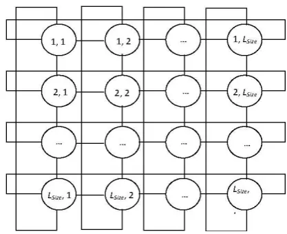
In TDLSMAPSO, all agents live in square lattice-like structured environment as in Fig. 3. In the environment L, each agent is placed on a lattice-point and each circle represents an agent. The size of L is L

size ×Lsize where Lsize is

an integer number. In TDLSMAPSO, number of particles and L should be same.

In CLSMAPSO, all agents live in cubic lattice-like structured environment as in Fig. 4. In the environment L, each agent is placed on a lattice-point and each circle represents an agent. The size of L is L

size ×Lsize ×Lsize where Lsize is an integer. In

CLSMAPSO, number of particles and L should be same.

Fig 3. Square Lattice structure of Multi agent system for TDLSMAPSO

Fig 4. Cubic lattice structure of multi agent system for CLSMAPSO

4.4.1.2

Definition of the Local Environment

Since each agent can only sense its neighbours, it is very essential to define the local environment. In this paper, in TDLSMAPSO, an agent λ located at (i,j) can have 8 neighbours (including agents at 4 sides and 4 corners ) as it can be seen from the lattice and in CLSMAPSO, an agent λ located at (i,j) can have 26 neighbours (including agents at 6 sides, 8 corners and 12 edges) as it can be seen from the lattice.

4.4.1.3

Behavioural rules for Agent

In TDLSMAPSO and CLSMAPSO, every agent competes and cooperates among its neighbours and makes use of evolution mechanism and knowledge of PSO and hence it diffuses all its information to whole environment. Based on the behaviours, the competition and cooperation operator were designed and are as follows.

4.5

Competition and Cooperation

Operator

Suppose that competition and cooperation operator ios performed on the agent λ located at (i,j) and λi,j=( λ1 ,λ2 ,

...λn) and Mini,j=( m1 ,m2 , ...mn) is the agent with

minimum fitness value among its neighbours, namely Mini,jϵNeighboursi,j. If agent λi,j satisfies the following

equation it is a winner otherwise it is a loser.

If λi,jis victorious, it can still live in the agent lattice. If λi,j is a

loser,it must die and its lattice-point will be occupied by Newi,j. The new agent Newi,j =(λ1

,

,λ2,, … … ,λ𝑛,) is determined

by the following strategy

(15)

5.

IMPLEMENTATION OF CLSMAPSO

FOR OPF PROBLEM

In TDLSMAPSO and CLSMAPSO, mainly the operators like competition and cooperation operators along with PSO operators were used to obtain the optimal solution in quick time with accuracy. The detailed algorithm of TDLSMAPSO and CLSMAPSO for OPF problem is as given below: 1. Input the required parameters and specify lower and

upper limits of variables. In OPF problem, PGi, i ϵ NG

except for slack bus are the variables.

2. Determine the fitness value of each agent i.e., Production cost or total Fuel cost, by Newton-Raphson power flow analysis results.

3. Sort the particles.

4. Create a lattice like environment L, and assign each agent (which is essentially a particle) on lattice point in the ascending order. Here each agent carries generation values of generators except slack bus power.

5. Increment the iteration counter

6. Carryout competition and cooperation operator on each agent and modify it.

7. Apply PSO mechanism to each agent and adjust its position using the equations related to velocity and position.

8. Determine the fitness value of each agent i.e., production cost, by Newton-Raphson power flow analysis results 9. Determine the best agent with minimum fitness value. 10. Sort the particles in ascending order.

11. Check for stopping condition (all the agents converge to a fitness value), if yes go to next step, else go to step (4). Print the agent and its fitness value.

6.

RESULTS AND DISCUSION

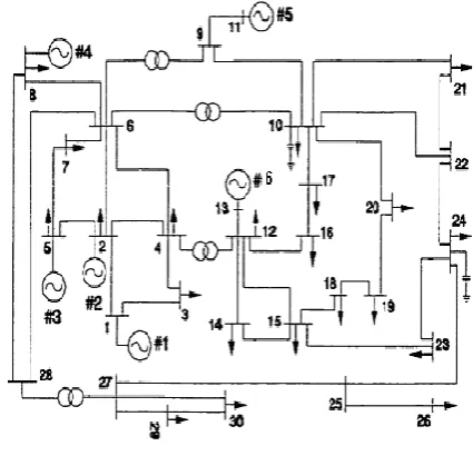
The algorithm is implemented in C programming language and executed on Intel Core 2 Duo system with 1GB RAM running on linux. To verify the performance of the CLSMAPSO algorithm, a standard representative system, i.e., IEEE30 bus systems has been taken as shown in Fig 5. The table 2 shows comparison of the results for CLSMAPSO, tdlsmapso and original PSO algorithm with constriction factor with different methods in the literature. For all the algorithms c1=0.6, c2=0.4, r1=0.6, r2=0.4 and inertia,ω=0.8. The number of particles for CLSMAPSO is 27 and for PSO it is 25.

Fig 5. Single line diagram of standard IEEE 30 bus system

Table1. Generator data with quadratic cost functions considered for IEEE 30 bus system

Bu s N o min G

P

P

Q

Q

1 50 200 -20 200 0 2.0 0.0037

5

2 20 80 -20 100 0 1.75 0.0175

5 15 50 -15 80 0 1.0 0.0625

8 10 35 -15 60 0 3.25 0.0083

4

11 10 30 -10 50 0 3.0 0.0250

13 12 40 -15 60 0 3.0 0.0250

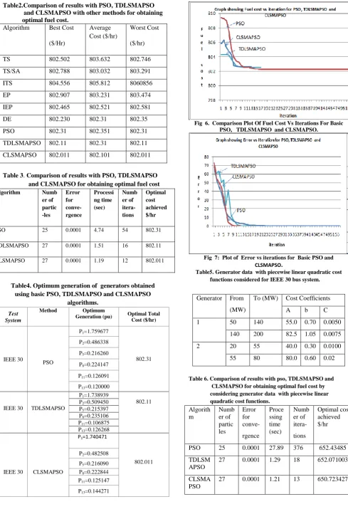
Table2.Comparison of results with PSO, TDLSMAPSO and CLSMAPSO with other methods for obtaining optimal fuel cost.

Algorithm Best Cost ($/Hr)

Average Cost ($/hr)

Worst Cost ($/hr)

TS 802.502 803.632 802.746

TS/SA 802.788 803.032 803.291

ITS 804.556 805.812 8060856

EP 802.907 803.231 803.474

IEP 802.465 802.521 802.581

DE 802.230 802.31 802.35

PSO 802.31 802.351 802.31

TDLSMAPSO 802.11 802.31 802.11

CLSMAPSO 802.011 802.101 802.011

Table 3. Comparison of results with PSO, TDLSMAPSO and CLSMAPSO for obtaining optimal fuel cost Algorithm Numb

er of partic -les

Error for conve-rgence

Processi ng time (sec)

Numb er of itera-tions

Optimal cost achieved $/hr

PSO 25 0.0001 4.74 54 802.31

TDLSMAPSO 27 0.0001 1.51 16 802.11

CLSMAPSO 27 0.0001 1.19 12 802.011

Table4. Optimum generation of generators obtained using basic PSO, TDLSMAPSO and CLSMAPSO

algorithms.

Test System

Method Optimum

Generation (pu) Optimal Total

Cost ($/hr)

PSO

P1=1.759677

802.31 IEEE 30

P2=0.486338

P5=0.216260

P8=0.224147

P11=0.126091

P13=0.120000

IEEE 30 TDLSMAPSO

P1=1.738939

802.11 P2=0.509450

P5=0.215397 P8=0.235106 P11=0.106875 P13=0.126268

P1=1.740471

P2=0.482508

P5=0.216090 802.011 IEEE 30 CLSMAPSO P8=0.222844

P11=0.125147

P13=0.144271

Fig 6. Comparison Plot Of Fuel Cost Vs Iterations For Basic PSO, TDLSMAPSO and CLSMAPSO.

Fig 7: Plot of Error vs iterations for Basic PSO and

CLSMAPSO.

Table5. Generator data with piecewise linear quadratic cost functions considered for IEEE 30 bus system.

Generator From (MW)

To (MW) Cost Coefficients

A b C

1 50 140 55.0 0.70 0.0050

140 200 82.5 1.05 0.0075

2 20 55 40.0 0.30 0.0100

55 80 80.0 0.60 0.02

Table 6. Comparison of results with pso, TDLSMAPSO and CLSMAPSO for obtaining optimal fuel cost by considering generator data with piecewise linear quadratic cost functions.

Algorith m

Numb er of partic les

Error for conve- rgence

Proce ssing time (sec)

Numb er of itera- tions

Optimal cost achieved $/hr

PSO 25 0.0001 27.89 376 652.43485 TDLSM

APSO

27 0.0001 1.29 18 652.071003

CLSMA PSO

Table7. Generator data with quadratic cost functions with multiple valve point loading effects considered for IEEE 30 bus system.

Gen min G

P

P

a B C d e

1 50 200 150.0 2.0 0.0016 50.0 0.063 2 20 80 25.0 2.5 0.0010 40.0 0.098

Table8. Comparison of results with PSO, TDLSMAPSO and CLSMAPSO for obtaining optimal fuel cost by considering generator data with quadratic cost functions by considering

mulltiple valvepoint loading effects.

Algorithm Num ber of partic les

Error for conve-

rgence

Proces sing time (sec)

Nu mb er of iter a-

tio ns

Optimal cost achieved $/hr

PSO 25 0.0001 11.125 147 919.707134

TDLSMAP SO

27 0.0001 1.12 13 919.624804

CLSMAPS O

27 0.0001 0.99 11 919.08384

7.

CONCLUSION

Based on multi agent systems, TDLSMAPSO and CLSMAPSO have been developed for solving Optimal power Flow problem (OPF) with security constraints. To the best of our knowledge, OPF problem has been solved by several methods in the literacy but these unique TDLSMAPSO and CLSMAPSO methods integrates the square and Cubic Lattice Structured multi agents respectively for TDLSMAPSO and CLSMAPSO with PSO using variable constriction factor to find the global or near global optimum point for OPF problem. IEEE 30 bus with different cost functions has been tested with PSO, TDLSMAPSO and CLSMAPSO methods and results are compared. From the results, TDLSMAPSO and CLSMAPSO converges to global optimum with more accuracy and within less time. From the results, CLSMAPSO converges to global optimum with an accuracy of 0.0001 and within less time. It can be observed that PSO is consuming more time and iterations to converge, where as TDLSMAPSO and CLSMAPSO were consuming less time and less number of iterations to obtain near optimum solution. Hence, we can say that TDLSMAPSO and CLSMAPSO algorithms were very fast and accurate. Moreover, from the literature it is observed that we have got the best optimal cost with PSO,TDLSMAPSO and CLSMAPSO. These algorithms are general and can be applied to other power system optimization problems.

8.

REFERENCES

[1] Hermann W. Dommel, and William F. Tinney,”optimal Power Flow Solutions”

[2] Sivasubramani.S, Shanti Swarup K, Multiagent Based Particle Swarm Optimization Approach to Economic Dispatch With Security Constraints December27-29‟2009, International Conference on Power systems, ,Kharagpur” .

[3] Bo Yang,Yuping ChenmZunlian Zhao and Qiye Han, “Solving Optimal Power Flow Problems with improved Particle Swarm Optimization”,Proceedings of 6th _world

congress on Intelligent Control and Automation,June 21-23,2006,Dalian,China.

[4] J. Nanda, D.P. Kothari, and S.C. Srivastava, “New optimal power dispatch using fletcher‟s quadratic programming method,” IEEE Proc C, pp. 153-161, 1989. [5] J. Nanda, and B.R. Narayanan, “Application of genetic algorithm to economic load dispatch with line flow constraints,” Int Journal of Electric Power Energy Systems, pp. 723-729, 2002.

[6] P. Somasundaram, and K. Kuppusamy, “Application of evolutionary programming to security constrained economic dispatch,” Electric Power and Energy Systems, pp. 343-351, 2005.

[7] J. Kennedy, and R. Eberhart, “Particle swarm optimization,” Proc IEEE Int Conf Neural Networks, Aust, pp. 1942-1948, 1995.

[8] R.C. Eberhart, and Y. Shi, “Comparing inertia weights and constriction factors in particle swarm optimization,” Proc Congr Evolutionary Computation, pp. 84-88, 2000. [9] J. B. Park, K.S. Lee, J.R. Shin, and K.Y. Lee, “A particle swarm optimization for economic dispatch with non-smooth cost functions,” IEEE Trans on Power Systems, pp. 34-42, 2005.

[10] K.S. Swarup, and P. Rohit Kumar, “A new evolutionary computation technique for economic dispatch with security constraints,” Electric Power and Energy Systems, pp. 273-283, 2006.

[11] M. Wooldridge, An introduction to multiagent system. New York: Wiley, 2002.

[12] W. Zhong, J. Liu, M. Xue, and L. Jiao, “ A multiagent genetic algorithm for global numerical optimization,” IEEE Trans on Sys, Man and Cybernatics, pp. 1128-1141, 2004.

[13] B. Zhao, C.X. Guo, and Y.J. Cao, “A multiagetn-based particle swarm optimzation approach for optimal reactive power dispatch,” IEEE Trans on Power Systems, pp. 1070-1078, 2005.

[14] Y. Wallach, Calculations and programs for power system networks. Englewood Cliffs, NJ: Prentice-Hall, 1986.

9.

AUTHORS PROFILE

K.Ravi Kumar received his B.Tech and M.Tech degrees in 1994 and 2005 respectively from JNTU college of Engineering, Hyderabad.Presently he is working as Associate Professor of Electrical and Electronics Engineering

Department at Vasavi college of

Engineering,Hyderabad,India. He is currently pursuing PhD degree in Power Systems at National Institute of Technology,Warangal,India. His fields of interest are Power system optimization,FACTS and Evolutionary Computation. S.Anand received his B.Tech degree in 2009 from Vasavi College of Engineering,Hyderabad. Currently he is working as a senoir software analyst at Intergraph consulting, Hyderabad. His fields of interest are Power system

optimization, FACTS, Evolutionary Computation and Power Electronics.