A Range Based GARCH Model for Forecasting Volatility

A Range-Based GARCH Model for

Forecasting Volatility

Mapa, Dennis S.

School of Statistics University of the Philippines Diliman, School of

Economics, University of the Philippines Diliman

December 2003

Online at

https://mpra.ub.uni-muenchen.de/21323/

Dennis S. Mapa1

ABSTRACT

A new variant of the ARCH class of models for forecasting the conditional variance, to be called the Generalized AutoRegressive Conditional Heteroskedasticity Parkinson Range (GARCH-PARK-R) Model, is proposed. The GARCH-PARK-R model, utilizing the extreme values, is a good alternative to the Realized Volatility that requires a large amount of intra-daily data, which remain relatively costly and are not readily available. The estimates of the GARCH-PARK-R model are derived using the Quasi-Maximum Likelihood Estimation (QMLE). The results suggest that the GARCH-PARK-R model is a good middle ground between intra-daily models, such as the Realized Volatility and inter-daily models, such as the ARCH class. The forecasting performance of the models is evaluated using the daily Philippine Peso-U.S. Dollar exchange rate from January 1997 to December 2003.

Key Words: Volatility, Parkinson Range, GARCH-PARK-R, QMLE

I. INTRODUCTION

Since the introduction of the seminal paper on AutoRegressive Conditional

Heteroskedasticity (ARCH) process of Robert Engle in 1982, researches on

financial econometrics have been dominated by extensions of the ARCH

process. One particular difficulty experienced in evaluating the various

ARCH-type of models is the fact that volatility is not directly measurable – the

conditional variance is unobservable. The absence of such a benchmark that we

can use to compare forecasts of the various models makes it difficult to identify

good models from bad ones.

Anderson and Bollerslev (1998) introduced the concept of “realized volatility”

from which evaluation of ARCH volatility models are to be made. Realized

volatility models are calculated from high-frequency intra-daily data, rather than

inter-daily data. In their seminal paper, Anderson and Bollerslev collected

information on the DM-Dollar and Yen-Dollar spot exchange rates for every

five-minute interval, resulting in a total of 288 5-five-minute observations per day! The 288

observations were then used to compute for the variance of the exchange rate of

a particular day. Although volatility is an instantaneous phenomenon, the concept

of realized volatility is by far the closest we have to a “model-free” measure of

volatility.

Obviously, there is a trade-off when one is interested in estimating the conditional

variance using realized volatility. While it may provide a model-free estimate of

the unknown conditional variance, the data requirement (getting observation

every 5 minutes, for instance) is simply enormous. In the case of the Philippines,

the Philippine Stock Exchange (PSE) starts trading at 9:30 a.m. up to 12:00

noon, for a total of 150 minutes of trading time or 30 5-minute observations.

Given the low market activity, it is highly probable that the price of a particular

stock will not move during that 5-minute period. The same problem might be

encountered in the foreign exchange market in the Philippine Dealing System

(PDS). Data problem may hinder the use of realized volatility for emerging

markets such as the Philippines.

An alternative approach to model volatility using intra-daily data is through the

use of the range, the difference between the highest and lowest values for the

day. The range is the popular measure of volatility (the standard deviation) in the

area of quality control. The range is convenient to use, especially for researchers

who do not have access to information on the trading floors of various markets,

since major newspapers normally report the highest and lowest values of assets

(stock prices, currencies, interest rates, etc.), together with the opening and

This paper proposes the use of the Range, specifically the Parkinson Range, in

estimating the conditional variance. The model will be called the Generalized

AutoRegressive Conditional Heteroskedasticity Parkinson Range

(GARCH-PARK-R) model. This paper is organized as follows: section 1 serves as the

introduction, section 2 discusses the ARCH process and its extensions. Section 3

introduces the concept of realized volatility. The GARCH-PARK-R model and the

estimation procedure are discussed in section 4. Section 5 provides the empirical

results and section 6 concludes.

II. The ARCH Process and its Extensions

In this section, the ARCH process will be defined and some of its important

properties discussed. Hopefully, doing it at this early stage will serve two

purposes. First is to acquaint the readers of the ARCH process for them to fully

appreciate the survey of the literature discussed. Secondly, for them to have a

better understanding of the important properties of the ARCH process that made

it very attractive in modeling financial time series.

Let {ut(θ), t ∈ (…,-1,0,1,…)} denote a discrete time stochastic process with the conditional mean and variance functions having parameterized by the finite

dimensional vector θ ∈Θ ⊆ℜm and let θo denote the true value of the parameter.

Let E[(•)| Ιt-1] or Et-1(•) denote the mathematical expectation conditioned on the

information available at time (t-1), Ιt-1.

Definition 1. In the relationship, ut = Ztσt, the stochastic process {ut(θ), t ∈ (-∞, ∞)} follows an ARCH process if:

b. Var (ut(θo) | Ιt-1) = σt2(θo) depends non-trivially on the sigma

field generated by the past observations, { ut-12(θo), ut-22(θo), …}.

σt2(θo) ≡ σt2 is the conditional variance of the process, conditioned on the

information set Ιt-1. The conditional variance is central to the ARCH process.

Letting Zt (θo) = ut (θo)/σt (θo), t = 1,2, … we have the standardized process { Zt

(θo) t ∈ (-∞, ∞)} and it follows that,

(i) E [Zt (θo) | Ιt-1] = 0 ∀ t

(ii) Var [Zt (θo) | Ιt-1] = 1 ∀ t

Thus, the conditional variance of Zt (.) is time invariant. Moreover, if we assume

that the conditional distribution of Zt(.) is time invariant with a finite fourth

moment, it follows from Jensen’s inequality that,

E(ut4) = E(Zt4)E(σt4) ≥ E(Zt4) [E(σt2)]2 = E(Zt4) [E(ut2)]2

with the last equality holding only when the conditional variance is constant.

Assuming that Zt(.) is normally distributed, it follows that the unconditional

distribution of ut is leptokurtic.

Engle (1982) has shown that for the first order or ARCH(1) process,

σt2 = αo + α1ut-12 (1)

the unconditional variance and the fourth moment for this process are,

1 0 2 1 ) ( α α − = t u E

(

)

The condition for the variance to be finite is that α1 < 1 and for the fourth

moment, 3α12 < 1.

It implies that E(ut4)/ E[(ut2)]2≥ E(Zt4). Thus, for the first order ARCH process,

3 ) 3 1 ( ) 1 ( 3 )) ( ( ) ( 2 1 2 1 2 2 4 > − − = α α t t u E u E

This result implies that the ARCH (1) process is a heavy-tailed distribution, that

is, the process generates data with fatter tails than the normal distribution. This

particular characteristic of the ARCH process is relevant in modeling financial

time series, like stock returns and asset prices, since these series tend to have

thick-tailed distributions.

In general, the ARCH (q) process can be defined as,

) 2 ( 2 2 2 2 2 1 1 2 q t q t t

t =ω+α u − +α u− + +α u−

σ L

For this model to be well defined and have a positive conditional variance almost

surely, the parameters must satisfy ω > 0 and α1, …, αq≥ 0. We will see later that

for the Generalized ARCH or the GARCH process, this condition can be made

Following the natural extension of the ARMA process as a parsimonious

representation of a higher order AR process, Bollerslev (1986) extended the work

of Engle to the Generalized ARCH or GARCH process. In the GARCH (p,q)

process defined as,

p j

q i

u

j i

q

i i t i p

j j t j t

, , 1 ,

, 1 0 ,

0 , 0

) 3 ( 1

2

1 2 2

K

K =

= ≥ ≥

>

∑ + ∑

+ =

= −

= −

β α

ω

α σ

β ω σ

the conditional variance is a linear function of q lags of the squares of the error

terms (ut2) or the ARCH terms (also referred to as the “news” from the past) and

p lags of the past values of the conditional variances (σt2) or the GARCH terms,

and a constant ω. The inequality restrictions are imposed to guarantee a positive

conditional variance, almost surely.

2.2.2. The Exponential GARCH (EGARCH) Process

The GARCH process being an infinite or a higher order representation of the

ARCH process captures the empirical regularities observed in the time series

data such as thick-tailed distributions and volatility clustering. However, the

GARCH process fails to explain the so-called “leverage effects” often observed in

financial time series. The concept of leverage effects, first observed by Black

(1976), refers to the tendency for changes in the stock prices to be negatively

correlated with changes in the stock volatility. In other words, the effect of a

shock on the volatility is asymmetric, or to put it differently, the impact of a “good

news” (positive lagged residual) is different from the impact of the “bad news”

The GARCH process, being symmetric, fails to capture this phenomenon since in

the model, the conditional variance is a function only of the magnitudes of the

lagged residuals and not their signs.

A model that accounts for an asymmetric response to a shock was credited to

Nelson (1991) and is called an Exponential GARCH or EGARCH model. The

specification for the conditional variance using the EGARCH (p,q) is,

k t

k t r

k k i

t i t q

i i p

j j t j t

u u

− − = − − =

= − + ∑ + ∑

∑ + =

σ γ σ

α σ

β ω σ

1 1

1

2 2_{) log( )} log(

The log of the conditional variance implies that the leverage effect is exponential

rather than quadratic. A commonly used model is the EGARCH (1,1) given by,

) 4 ( )

log( )

log(

1 1 2

1 1

1 1 1 0 2

− − −

−

− _{+ +}

+ =

t t t

t t t

u u

σ γ σ

β σ

α α σ

The presence of the leverage effects is accounted for by γ, which makes the

model asymmetric. The motivation behind having an asymmetric model for

volatility is that it allows the volatility to respond more quickly to falls in the prices

(bad news) rather than to the corresponding increases (good news).

2.2.3. The Threshold GARCH (TARCH) Process

Another model than accounts for the asymmetric effect of the “news” is the

Threshold GARCH or TARCH model due independently to Zakoïan (1994) and

Glosten, Jaganathan and Runkle (1993). The TARCH (p,q) specification is given

⎩ ⎨

⎧ < =

∑ + ∑

+ ∑

+ =

− −

− − − = − = − =

otherwise u if I

where

I u u

t k

t

k t k t r

k k i

t q

i i j

t p

j j t

0

0 1

,

) 5 (

2

1 2

1 2

1

2 _{ω β σ α γ}

σ

In the TARCH model, “good news”, ut-i > 0 and “bad news”, ut-i < 0 have different

effects on the conditional variance. When γk ≠ 0, we conclude that the news

impact is asymmetric and that there is a presence of leverage effects. When γk =

0 for all k, the TARCH model is equivalent to the GARCH model. The difference

between the TARCH and the EGARCH models is that in the former the leverage

effect is quadratic while in the latter, the leverage effect is exponential.

2.2.4. The Power ARCH (PARCH) Process

Most of the ARCH-type of models discussed so far deal with the conditional

variance in the specification. However, when one talks of volatility the appropriate

measure is the standard deviation rather than the variance as noted by

Barndorff-Nielsen and Shephard (2002). A GARCH model using the standard

deviation was introduced independently by Taylor (1986) and Schwert (1989). In

these models, the conditional standard deviation as a measure of volatility is

being modeled instead of the conditional variance. This class of models is

generalized by Ding et al. (1993) using the Power ARCH or PARCH model. The

. ,

0 ,

, 2 , 1 1

, 0

,

) 6 ( )

( 1 1

p r and r i for and

r i

for where

u u

i i

i t i i t q

i i j

t p

j j t

≤ >

= =

≤ >

− ∑

+ ∑

+

= _{− −}

= − =

γ γ

δ

γ α

σ β ω

σδ δ δ

K

Note that in the PARCH model, γ ≠ 0 implies asymmetric effects. The PARCH

model reduces to the GARCH model when δ = 2 and γi = 0 for all i.

III. The Realized Volatility

Let Pn,t denote the price of an asset (say US$ 1 in Philippine Peso) at time n ≥ 0

at day t, where n = 1,2,…,N and t=1,2,…,T. Note that when n=1, Pt is simply the

inter-daily price of the asset (normally recorded as the closing price). Let pn,t =

log(Pn,t), denote the natural logarithm of the price of the asset. The observed

discrete time series of continuously compounded returns with N observations per

day is given by,

) 7 (

, 1 ,

,t nt n t

n p p

r = − ₋

When n=1, we simply ignore the subscript n and rt = pt – pt-1 = log(Pt) – log(Pt-1)

where t= 2,…,T. In this case, rt is the time series of daily return and is also the

covariance-stationary series. In (7), we assume that:

(a) E(rn,t) = 0

(b) E(rn,t rm,s) = 0 for n ≠ m and t ≠ s

(c) E(rn,t2 rm,s2) < ∞ for n,m,s,t

Assumption (a) implies that the mean return which follows from the fact that the

) 8 ( ) , 0 ( . . . ~

| ₁ 2

, ,

, 1

,t n t nt nt t t

n p where I iid

p = ₋ +ε ε ₋ σ

Following (8), rn,t = pn,t – pn-1,t = εn,t and thus, E(rn,t) = E(εn,t) = 0. Assumption (b)

follows from the fact that εn,t are i.i.d. and from (a) which gives us E(rn,t rm,s)=E(εn,t

εm,s) = 0. Assumption (c) states that the variances and co-variances of the squared returns exist and are finite. This follows from the fact that E(rn,t2

rm,s2)=E(εn,t2εm,s2) < ∞ for n,m,s,t.

From (7), the continuously compounded daily return (Campbell, Lo, and

Mackinlay, 1997 p.11) is given by,

)

9

(

∑

=

n nt

t

r

r

and the continuously compounded daily squared returns is,

) 10 (

2 _,

1 1 , 1

2 ,

, 1 1 , 1 2 , 2 1 , 2 t n m N n N n m nt N

n nt

t m N

n N

m nt N

n nt N

n nt t r r r r r r r r − = = + = = = = = ∑ ∑ + ∑ = ∑ ∑ + ∑ = ⎟ ⎠ ⎞ ⎜ ⎝ ⎛ ∑ =

Note that σt2 = Var(rt) = E(rt2) since E(rt) = 0. From (10) and using assumption (b)

of (7) above, we have,

( )

n nt t t t t r s where s E r E 1 2 , 2 2 2

2 _{( ) (11)}

σ

Thus, the sum of the intra-daily squared returns is an unbiased estimator of the

the realized volatility (also called the realized variance by Barndorff-Nielsen and

Shephard (2002)). Given enough observations for a given trading day, the

realized volatility can be computed and is a model-free estimate of the

conditional variance. The properties of the realized volatility are discussed in

Anderson, Bollerslev, Diebold and Labys (1999). In particular, the authors found

that the realized volatility is a consistent estimator of the daily population

variance, σt2.

IV. The GARCH-PARK-R Model

While the concept of realized volatility does provide a highly efficient way of

estimating the unknown conditional variance, the problem of generating

information on the price of an asset every five minutes or so is simply enormous.

An alternative measure is to use extreme values, the highest and lowest prices of

an asset, to produce two intra-daily observations. The range, the difference

between the highest and lowest log prices, is a good proxy for volatility. The

range has the advantage of being available for researchers since high and low

prices are available daily for a variety of financial time series such as price of

individual stock, composite indices, Treasury bill rates, lending rates, currency

prices and the like.

The log range, Rt, is defined as,

) 12 ( ,

2 , 1 )

log( ) log(

), 1 ( ), (

), 1 ( ),

(

T t

p p

P P

R

t t

N

t t

N t

K

= −

=

− =

where P(N),t is the highest price of the asset at day (or time) t and P(1),t is the

lowest price of the asset at day t.

The log range is superior over the usual measure of volatility based on daily data,

noted that the log range is a better measure of volatility in the sense that the log

range has fewer measurement errors compared to the squared-returns. For

instance, on a given day, the price of an asset fluctuates substantially throughout

the day but its closing price happens to be very close to the previous closing

price. If we use the inter-daily squared return, the value will be small despite the

large intra-daily price fluctuations. The log range, using the highest and lowest

values, reflects a more precise price fluctuations and can indicate that the

volatility for the day is high.

Moreover, the log range can be approximated by a Gaussian distribution quite

well. The distribution of the range was first derived by Feller (1951) using a

drift-less Brownian motion process.

As compared to the realized volatility, the log range has the advantage of being

robust to certain market microstructure effects. These microstructure effects,

such as the bid-ask spread, are noises that can affect the features of the

time-series. The bid-ask spread is a common type of microstructure effect. Most

markets require liquidity, giving way to a practice of granting monopoly rights to

the so-called “market makers.” Such monopoly rights, granted by the exchange,

allow the market makers to post different prices for buying and selling, they buy

at a bid price Pb and sell at a higher price Pa. The difference in the prices, Pa – Pb

is known as the spread. Although in practice, such spread is rather small, its

presence increases the volatility of the intra-daily squared returns, the input in the

realized volatility, making the estimates biased upward. The log range, on the

other hand, is not seriously affected by the bid-ask spread. There are other

factors that create unnecessary noise in the intra-daily realized volatility such as

regulatory rules imposed on the market. One such rule is the lifting of trading

restrictions in the foreign exchange market for Japanese banks during the Tokyo

lunch period resulting to higher volatility as documented by Anderson, Bollerslev

Parkinson (1980) was the first to make use of the range in measuring volatility in

the financial market. Parkinson developed the PARK daily volatility estimator

based on the assumption that the intra-daily prices follow as Brownian motion.

This study will make use of the PARK Range in modeling time-varying volatility.

The model will be called the Generalized Auto-Regressive Conditional

Heteroskedasticity Parkinson Range (GARCH-PARK-R) model.

Consider the covariance-stationary time series {Rpt} where,

) 13 ( , , 2 , 1 )

2 log( 4

) log( )

log( _{( ), (1),}

T t

P P

R_P N t t

t = K

− =

RPt is the PARK-Range of the asset at time t. Moreover, let RPt ≥ 0 for all t and

that P(RPt <δ| RPt-1, RPt-2,…) > 0 for any δ > 0 and for all t. This condition states

that the probability of observing zeros or near zeros in RPt is greater than zero.

Let,

μt = E[RPt| It-1] be the conditional mean of the PARK range and

σt2 = Var[RPt|It-1] be the conditional variance of the PARK range

The motivation behind the GARCH-PARK-R model is the Auto-Regressive

Conditional Duration (ACD) model of Engle and Russel (1998) used to model

Let, ) 14 ( ) , 1 ( ~ | 1 1 2 1 j t p j j P q j j t t t t t t P j t t R and iid I where R − = = − ∑ + ∑ + = =

− β μ α ω μ φ ε ε μ

The model in (14) is known as the GARCH-PARK-R process of orders p and q.

The mean and variance of the PARK range are given by,

( )

The GARCH-PARK-R model is similar to the Conditional Auto-Regressive Range

(CARR) model suggested by Chou (2003). Two differences between this study

and that of Chou’s are to be clarified. First, this study uses the Parkinson range

to study volatility instead of the usual log range (Chou’s measure). The Parkinson

range has been found to be a better estimator of volatility (standard deviation).

The second difference is the use of the data, this study makes use of the daily

data while Chou’s paper used weekly data. Weekly data may have distorted

estimates due to the presence of aggregation effect that is why the author of this

paper used the daily data instead.

For the density function of εt in (14), this study follows the suggestion of Engle

and Russel (1998) and Engle and Gallo (2003) of using the gamma density,

( )

1 ) |

( ₁ 1

⎭ ⎬ ⎫ ⎩ ⎨ ⎧ − Γ ⎟ ⎠ ⎞ ⎜ ⎝ ⎛ = −

− β_α ε ε_β

Since E(εt) = αβ = 1 (by assumption in (14)), it implies that α = 1/β. Thus (16)

now becomes,

( )

{

}

( )

( )

( )

( )

( )

( )

exp 1 exp 1 | ) | ( exp ) | ( 1 1 1 1 1 1 1 ⎪⎭ ⎪ ⎬ ⎫ ⎪⎩ ⎪ ⎨ ⎧ ⎟⎟ ⎠ ⎞ ⎜⎜ ⎝ ⎛ − Γ ⎟ ⎠ ⎞ ⎜ ⎝ ⎛ = ⎪⎭ ⎪ ⎬ ⎫ ⎪⎩ ⎪ ⎨ ⎧ ⎟ ⎟ ⎠ ⎞ ⎜ ⎜ ⎝ ⎛ − Γ = ⎪⎭ ⎪ ⎬ ⎫ ⎪⎩ ⎪ ⎨ ⎧ ⎟ ⎟ ⎠ ⎞ ⎜ ⎜ ⎝ ⎛ − ⎟ ⎟ ⎠ ⎞ ⎜ ⎜ ⎝ ⎛ Γ = ⎟ ⎟ ⎠ ⎞ ⎜ ⎜ ⎝ ⎛ = ⇒ − Γ = − − − − − − − − t P P t t P t P t P t P t t P t P t t t t t t t t t t t t R R R R R R I R f I R f I f μ α α μ α μ α μ α α μ α μ α α μ αε ε α α ε α α α α α α α α α

From (17), the conditional mean and variances of RPt are,

(

)

( )

The density function in (17) approaches the Gaussian density as α increases.

Moreover, the likelihood function is given by,

( )

( )

( )

1 ⎥ ⎥ ⎦ ⎤ ⎢ ⎢ ⎣ ⎡ ⎪⎭ ⎪ ⎬ ⎫ ⎪⎩ ⎪ ⎨ ⎧ ⎟ ⎟ ⎠ ⎞ ⎜ ⎜ ⎝ ⎛ − Γ ∏ = − − = _t P t P T t t t R R L μ α μ α α α α α

If the parameter of interest are only those that define μt in (14), denoted by μt(θ),

) , ( ) 19 ( ) ( )) ( log( ) log( log 1 1 1 t t t P T t t P t T t T t t P t R where R R L α γ γ θ μ θ μ α γ μ α μ α γ = ∑ ⎥ ⎦ ⎤ ⎢ ⎣ ⎡ + − = ∑ ∑ _⎟⎟ ⎠ ⎞ ⎜ ⎜ ⎝ ⎛ − − = = = =

Taking the derivative of the log likelihood function with respect to θ, we have,

) 20 ( 0 ) ( ) ( ) ( 0 ) ( ) ( 1 ) ( 0 ) ( ) ( ) ( ) ( 1 ) log( 1 2 1 2 1 2 = ∂ ∂ ∑ ⎥ ⎥ ⎦ ⎤ ⎢ ⎢ ⎣ ⎡ − ⇒ = ∂ ∂ ∑ ⎥ ⎥ ⎦ ⎤ ⎢ ⎢ ⎣ ⎡ − ⇒ = ∑ ⎥ ⎥ ⎦ ⎤ ⎢ ⎢ ⎣ ⎡ ∂ ∂ − ∂ ∂ − = ∂ ∂ = = = θ θ μ θ μ θ μ θ θ μ θ μ θ μ θ θ μ θ μ θ θ μ θ μ α θ t T t _t t P t T

t t t

P T t t t P t t t t t R R R L

The parameter vector θ in (20) can be estimated numerically using some iterative

algorithms such as the Marquardt or the BHHH.

An easier way of estimating the parameter vector θ is to apply the method of

estimating the parameters of a GARCH (p,q) process. Recall that in the GARCH

(p,q) process discussed in section 2,

∑ + ∑ + = = = − = − q

i i t i p

For the GARCH-PARK-R process let,

(

)

( )

(

)

( )

) 14 ( |

0 |

) 1 , 0 ( ~

1 1

2 1

1

in given R

with

E I

R Var and

E I

R E

iid R

j t p

j j P

q

j j t

t t t t

P

t t t

P

t t

t P

j t t t

t

− = =

− −

∑ + ∑

+ =

= =

= =

=

− β μ α

ω μ

μ ν μ ν μ

ν ν

μ

Thus, an analogous method of estimating the parameter vector θ is to estimate

the variance equation for the positive square root of the PARK R using GARCH

(p,q) specification with zero in the mean specification. The Quasi-Maximum

Likelihood estimators are consistent and distributed as Gaussian asymptotically

even if the probability density function of the error is mis-specified following the

results of Lee and Hansen and Lumsdaine for the GARCH (1,1) and Berkes et al

for the GARCH (p,q) process. Obviously, if the correct specification is satisfied,

for instance using the gamma distribution, the QMLE is the MLE and the

estimators are asymptotically efficient. Therefore, a trade-off has to be made.

This study will make use of the QMLE and aspire for consistency and asymptotic

normality of the estimators. The data and the results of the empirical analysis are

discussed in the next chapter.

V. Empirical Results

This chapter discusses the results of forecasting the conditional variance using

the different ARCH and GARCH-PARK-R models. In this study, a total of 77

models were estimated: 68 ARCH-type models and 9 GARCH-PARK-R models.

Table 1A. Specification for ARCH-type Models *

Model Specification Model Specification

1 ARCH (1) 10 TARCH (1,1)

2 GARCH (1,1) 11 TARCH (1,2)

3 GARCH (1,2) 12 TARCH (2,1)

4 GARCH (2,1) 13 TARCH (2,2)

5 GARCH (2,2) 14 PARCH (1,1)

6 EGARCH (1,1) 15 PARCH (1,2)

7 EGARCH (1,2) 16 PARCH (2,1)

8 EGARCH (2,1) 17 PARCH (2,2)

9 EGARCH (2,2)

* The 17 models are estimated via the MLE using the Gaussian, Student’s t and the Generalized Error Distribution and using the QMLE resulting to 68 models.

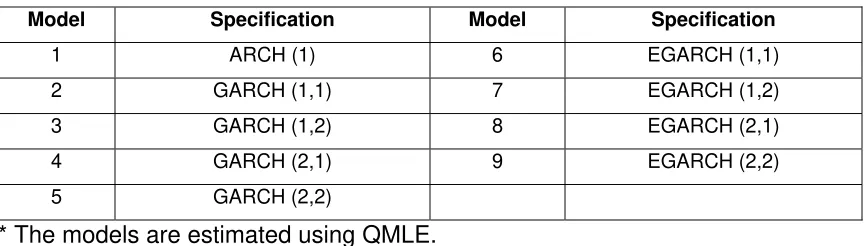
Table 1B. Specification for GARCH PARK R Models*

Model Specification Model Specification

1 ARCH (1) 6 EGARCH (1,1)

2 GARCH (1,1) 7 EGARCH (1,2)

3 GARCH (1,2) 8 EGARCH (2,1)

4 GARCH (2,1) 9 EGARCH (2,2)

5 GARCH (2,2)

* The models are estimated using QMLE.

These models were estimated to fit the daily returns of the peso-dollar exchange

rate from January 02, 1997 to December 05, 2003, a total of 1730 observations.

Following the approach of Hansen and Lunde (2001), the time series was divided

into two sets, an estimation period and an evaluation period.

t

₁

₄₂

₄₃

K

_{1 K}

₄₂

₄

₃

period evaluation period

estimation

n

,

,

2

,

1

0

,

,

1

T

−

The parameters of the volatility models are estimated using the first T inter-daily

observations and the estimates of the parameters are used to make forecasts of

for the remaining n periods. The estimation period made use of daily returns from

January 02, 1997 to December 27, 2002, a total of 1493 observations.

In the evaluation period the daily volatility is estimated using the square of the

Parkinson R, defined in (31). The square of the PARK R serves as the proxy for

the unknown conditional variance. The evaluation period makes use of daily

returns from January 02, 2003 to December 05, 2003, a total of 237

observations.

5.2. Loss Functions

Let h denote the number of competing forecasting models. The jth model provides

a sequence of forecasts for the conditional variance,

h j

n j j

j , ˆ , , ˆ 1,2, , ˆ2_,1 σ2_,2 K σ2_, = K

σ

that will be compared to the square of the Parkinson range, the proxy of the

intra-daily calculated volatility,

n P

P R

R2 , , 2

1 K

The forecast of jth model leads to the observed loss,

237 ,..., 2 , 1 77

,..., 2 , 1 ) , ˆ ( 2_, 2

, R j= and t=

L

t

In this study, five (5) different loss functions are used to evaluate the forecasting

performance of the different models. The loss functions are:

(

)

(

)

[

]

t P t

n t t n t t n t t n

t P t

t t P t P t P t ∑ = ∑ − = ∑ ⎟ ⎠ ⎞ ⎜ ⎝ ⎛ ₋ = ∑ − = ∑ − = = = = = = σ σ σ σ σ

The criteria (21) to (24) are the usual mean absolute deviations and mean square

errors using the forecasts of the conditional standard deviation and the

conditional variance.

Criterion (25) is equivalent to the R2 criterion using the regression equation,

237 , , 2 , 1 ) ˆ log( )

log(R_P2 =a+b _t2 + _t t= K

discussed in Engle and Patton (2001) and Taylor (1999).

The results of the forecasting performance are provided in Table 2 of the

Appendix of this study. The “best” 10 models are shown in Table 3 below. The

best over-all ARCH model is the TARCH (2,2) model with the Student’s t as the

underlying distribution. The second “best” model is the PARCH (2,2) model, also

using the Student’s t distribution.

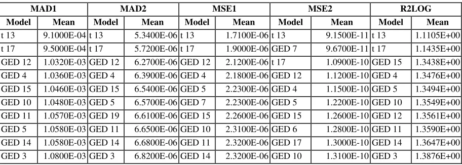
Table 3. Forecasting Performance of the Top 10 ARCH Models

MAD1 MAD2 MSE1 MSE2 R2LOG Model Mean Model Mean Model Mean Model Mean Model Mean

t 13 9.1000E-04 t 13 5.3400E-06 t 13 1.7100E-06 t 13 9.1500E-11 t 13 1.1105E+00 t 17 9.5000E-04 t 17 5.7200E-06 t 17 1.9000E-06 GED 7 9.6700E-11 t 17 1.1435E+00 GED 12 1.0320E-03 GED 12 6.2700E-06 GED 12 2.1200E-06 t 17 1.0900E-10 GED 15 1.3438E+00 GED 4 1.0360E-03 GED 4 6.3900E-06 GED 4 2.1800E-06 GED 12 1.1200E-10 GED 4 1.3476E+00 GED 15 1.0460E-03 GED 15 6.5400E-06 GED 5 2.2300E-06 GED 4 1.1500E-10 GED 5 1.3494E+00 GED 10 1.0480E-03 GED 5 6.5700E-06 GED 7 2.2300E-06 GED 5 1.2200E-10 GED 10 1.3549E+00 GED 11 1.0570E-03 GED 19 6.6100E-06 GED 15 2.2600E-06 GED 15 1.2600E-10 GED 12 1.3561E+00 GED 5 1.0580E-03 GED 11 6.6500E-06 GED 10 2.3100E-06 GED 6 1.2800E-10 GED 11 1.3590E+00 GED 14 1.0580E-03 GED 14 6.6800E-06 GED 11 2.3200E-06 GED 17 1.3000E-10 GED 14 1.3647E+00 GED 3 1.0800E-03 GED 3 6.8200E-06 GED 14 2.3200E-06 GED 10 1.3100E-10 GED 3 1.3876E+00

From Table 3, it is interesting to note that models using the Generalized Error

Distribution performed relatively well using the five forecasting criteria, with 8 out

of 17 models landing in the top 10 models. In general, the models with relatively

superior forecasting performance, using the peso-dollar exchange rate, are those

that accommodate the leverage effects such as the TARCH, PARCH and

EGARCH. However, while the correct specification of the volatility is important,

one must also consider the distribution used in estimating the parameters of the

model.

The results in Table 2 showed that volatility models that assumed the Gaussian

distribution or those that used the QMLE performed worst compared to models

important to correctly specify the entire distribution and not only to focus on the

specification of the volatility, even if it is the object of interest. A similar

observation was made in the study of Hansen and Lunde (2001).

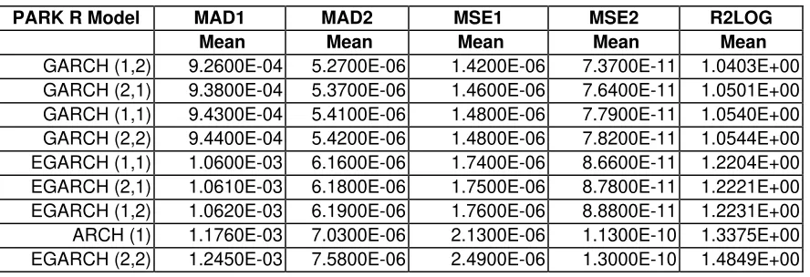
Using the five criteria discussed above the forecasting performance of the

GARCH – PARK – R models are given in Table 4. The top three models are

GARCH (1,2), (2,1) and (1,1). It should be noted that while the GARCH (1,2) and

the GARCH (2,1) have outperformed, albeit slightly, the GARCH (1,1), the latter

is preferred since the coefficients α and β are significantly different from zero.

Table 4. Forecasting Performance of the GARCH-PARK-R Models

PARK R Model MAD1 MAD2 MSE1 MSE2 R2LOG

Mean Mean Mean Mean Mean

GARCH (1,2) 9.2600E-04 5.2700E-06 1.4200E-06 7.3700E-11 1.0403E+00 GARCH (2,1) 9.3800E-04 5.3700E-06 1.4600E-06 7.6400E-11 1.0501E+00 GARCH (1,1) 9.4300E-04 5.4100E-06 1.4800E-06 7.7900E-11 1.0540E+00 GARCH (2,2) 9.4400E-04 5.4200E-06 1.4800E-06 7.8200E-11 1.0544E+00 EGARCH (1,1) 1.0600E-03 6.1600E-06 1.7400E-06 8.6600E-11 1.2204E+00 EGARCH (2,1) 1.0610E-03 6.1800E-06 1.7500E-06 8.7800E-11 1.2221E+00 EGARCH (1,2) 1.0620E-03 6.1900E-06 1.7600E-06 8.8800E-11 1.2231E+00 ARCH (1) 1.1760E-03 7.0300E-06 2.1300E-06 1.1300E-10 1.3375E+00 EGARCH (2,2) 1.2450E-03 7.5800E-06 2.4900E-06 1.3000E-10 1.4849E+00

As expected, the GARCH-PARK-R models performed better than most of the

ARCH-type models. This is expected since the proxy for the conditional variance

in the evaluation period is the square of the Parkinson range. However, it is

interesting to note that the forecasting performance of the “best” ARCH-type

model, the TARCH (2,2) model with a student’s t distribution, is relatively near

the “best” GARCH-PARK-R model. The results somewhat provide an assurance

that volatility models using inter-daily data can forecast the conditional variance

VI. Conclusion

This paper introduced a relatively simple, yet efficient, model to describe the

variation in volatility of the peso-dollar exchange rate using intra-daily returns.

The Generalized Auto-Regressive Conditional Heteroskedasticity Parkinson

Range (GARCH-PARK-R) model can actually produce volatility estimates that

are relatively superior than the ARCH class of models using inter-daily returns.

The GARCH-PARK-R model is a good alternative to the so-called Realized

Volatility that makes use of large quantity of intra-daily data, something that is

difficult to obtain in emerging markets such as the Philippines.

REFERENCES

Andersen T.G. and Bollerslev, T. (1998), “Answering the Skeptics: Yes, Standard Volatility Models do Provide Accurate Forecasts”, International Economic Review, 39, 885-905.

Anderson, T., Bollerslev, T., Diebold, F. X., and Labys, P., “The Distribution of Exchange Rate Volatility”, working paper 6961, National Bureau of Economic Research, February 1999.

Barndorff-Nielsen, O. E. and Shephard, N. (2002), “Estimating Quadratic Variation using Realized Variance”, Journal of Applied Econometrics, 17, 457-477.

Bollerslev, T. (1986), “Generalized Autoregressive Conditional Heteroskedasticity”, Journal of Econometrics, 31, 307-327.

Bollerslev, T. and Wooldridge, J. M. (1992), “Quasi Maximum Likelihood Estimation and Inference in Dynamic Models with Time Varying Covariances”,

Economic Reviews, 11, 143-172.

Busch, T., “Finite Sample Properties of GARCH Quasi-Maximum Likelihood Estimators and Related Test Statistics”, working paper, University of Aarhus, October 2003.

Chou, R. (2003), “Forecasting Financial Volatilities with Extreme Values: The Conditional Autoregressive Range (CARR) Model”, paper, Institute of Economics, Academia Sinica.

Ding, Z., Engle, R.F., and Granger, C. W. J. (1993) “Long Memory Properties of Stock Market Returns and a New Model”, Journal of Empirical Finance, 1, 83-106.

Engle, R. F. (1982), “Autoregressive Conditional Heteroscedasticity with Estimates of the Variance of United Kingdom Inflation”, Econometrica, 50, 987-1007.

Engle, R. F. (2002), “New Frontiers for ARCH Models”, Journal of Applied Econometrics, 17, 425-446.

Engle, R. F. and Gallo, G. (2003), “A Multiple Indicators Model for Volatility Using Intra-Daily Data”, working paper 10117, National Bureau of Economic Research, November 2003.

Engle, R. F. and Patton, A. J. (2001), “What Good is a Volatility Model?”

unpublished manuscript, Department of Finance, Stern School of Business, New York University.

Engle, R. F. and Russell, J. (1998), “Autoregressive Conditional Duration: A New Model for Irregularly Spaced Transaction Data”, Econometrica, 66, 1127-1162.

Glosten, L. R., Jagannathan, R., and Runkle, D. (1993) “On the relation between the Expected Value and the Volatility of the Nominal Excess Return on Stocks”, Journal of Finance, 48, 1779-1801.

Hansen, P. and Lunde, A. (2001), “A Forecast Comparison of Volatility Models: Does anything Beat a GARCH (1,1)?”, working paper, Department of Economics, Brown University, November 2001.

Lee, S. and Hansen B. E. (1994), “Asymptotic Theory for the GARCH (1,1) Quasi-Maximum Likelihood Estimator”, Economic Theory, 10, 29-52.

Lumsdaine, R. L. (1996), “Consistency and Asymptotic Normality of the Quasi-Maximum Likelihood Estimator in IGARCH (1,1) and Covariance Stationarity GARCH (1,1) Models”, Econometrica, 64, 575, 596.

Parkinson, M. (1980), “The Extreme Value Method for Estimating the Variance of the Rate of Return”, Journal of Business, 53, 61-65.

Taylor, J. W. (1999), “Evaluating Volatility and Interval Forecasts”, Journal of Forecasting, 18, 11-128.