Genetic Algorithm: An approach to Velocity Control of an Electric DC Motor

Genetic Algorithm: An approach to Velocity Control of

an Electric DC Motor

M. B. Anandaraju

HOD, Deptt of ECE, BGSIT, B.G.Nagara, Mandya, Dist.

Dr. P.S. Puttaswamy

Prof, Deptt of E&E, PESCE, Mandya.

Jaswant Singh Rajpurohit

Technical Director, Planet-I Technologies, Bangalore.

ABSTRACT

DC motor is a vital component in most of the process control industries. PID controllers are extensively used in DC motors for speed as well as position control. Tuning of PID controller parameters is an iterative process and needs complete optimization to achieve the desired performance. Genetic algorithm (GA) which is a well established tool for optimization has been used to extract PID controller parameters for the velocity control of the DC motor. Different error models are used for evaluating the fitness function. Velocity control is demonstrated using M ATLAB/SIM ULINK modeling.

Keywords

Component; DC motor, PID, Genetic Algorithm, Fitness Function

1.

INTRODUCTION

M echanical applications based on electric motors demand high speed accuracies [1]. Drive design for such systems is a complicated and involved process given the number of parameter optimizations involved. M any modern control methodologies like adaptive control [2], nonlinear control [3], optimal control [4] have been studied and attempted to deal with different types of motor controls. These approaches are mathematically complex and complicated to implement. M otor control based on proportional, integral and derivative (PID) controllers has been largely studied and implemented with success.

The present work deals with controlling the time domain performance parameters of a DC motor. The work based on developing a mathematical model of the DC motor which is then integrated with PID controller using SIM ULINK. Determination of the controller gains that maximizes or minimizes a performance specification is a complex, constrained optimization problem.

Genetic Algorithms (GAs) [5] present a way to solve such complex optimization problems. GAs has been used extensively in adaptive control of continuous and discrete-time [6], decentralized PI controls [7] as well as optimal control problems [8]. In the present work GA is used as a computing tool to solve

2. MODELING A DC MOTOR

2.1

Modeling Scheme

Electric DC motor coverts electrical energy to mechanical energy using the electromagnetic induction principle [9]. To achieve velocity control of a DC motor, the primary requirement is to model the DC motor system itself [10]. In control systems terminolo gy it is referred to as plant modeling. The major steps in developing a DC motor model are as follows:

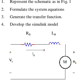
1. Represent the schematic as in Fig. 1

2. Formulate the system equations

3. Generate the transfer function.

4. Develop the simulink model

Ra La

Fig 1: Armature S chematic of a DC Motor

By applying a voltage to the coil, it causes a current to flow which produces a proportional torque. This in turn accelerates the armature. As the armature gathers speed, a proportional electromagnetic field is generated which tends to oppose the current. Eventually, the rotor gathers sufficient speed such that the back electromagnetic field just equals the applied voltage. In the steady state, when = , no current flows in the coil thus there is no further acceleration and the rotor turns at a constant speed.

inductance; if the current in the coil changes then there will be an induced back emf which opposes that change.

2.2

System Equations

Fig. 1 shows the schematic representation of a DC motor Ra,

L

and

e

back emf, respectively. The motor torque force required to rotate the object about its axis is related to the armature current,

by torque constant K represented as:

The back emf is voltage or electromagnetic force that pushes

against the current which is induced by armature is related to angular velocity as represented as:

In mechanical domain, if J is the rotational moment of inertia of motor, is the motor angular velocity, is the net

torque where the electromagnetic torque and load torque,

the torque equation in terms of moment of inertia we can write as:

Combining Newton’s law and Kirchhoff’s law we can write:

From the above equations, we can derive the s-domain transfer function of the motor which can be used for complex frequency functions:

To find the transfer function we required

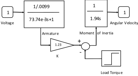
Fig2: Block Diagram of a DC Motor

3

GENETIC ALGORITHM

Genetic algorithm (GA) is a heuristic mimicking the natural evolution process and is routinely used to generate useful solutions to optimization problems. In this work the genetic algorithm is used to derive the PID controller parameters by optimizing the error in the DC motor angular velocity.

In GA [5, 12], a population of strings called chromosomes encodes the possible solutions of an optimization problem and evolves for a better solution by process of reproduction. The process of evolution starts from a population of randomly generated individuals. Optimization is achieved in generations where in each generation, the fitness function evaluates each individual in the population and multiple individuals are selected stochastically based on their fitness. These selected individuals are modified to form a new population. The algorithm terminates when either a maximum number of generations has been produced, or a satisfactory fitness level has been reached for the population. The various steps in GA based optimization are detailed below:

3.1. Initialization

From the initial population few individual solutions are generated. The population is generated randomly, covering the entire range of possible solutions.

3.2. Selection

In each generation, individual solutions are selected by evaluating the fitness function and the fitter solutions have a higher probability of selection

+

PID

M Current

Controller

H- Bridge Convertor

Current Sensor

Techo Feedback I/P An gular

Velocity

+

-

-

3.3. Reproduction

Next set of population for the successive generation is generated by a process called reproduction and involves crossover (recombination) and mutation. This result s in a new set of population derived from the fitter solutions of the previous population. Generally the average fitness of the population is heightened as compared to the population of the previous population.

3.4. Termination

The process of optimization is halted once a termination condition is achieved. The termination condition can be either the number of generations or the solution satisfying an optimum criterion.

4

MATLAB MODELING

4.1

Motor model

M otor model is developed using SIM ULINK/M ATLAB Fig 2. As the major objective of this work is to achieve velocity control, the GA optimization has been attempted for the PID controller for the velocity loop. The parameters for PID controller are the individuals in the GA population. For each individual, the SIM ULINK model is run and the error is computed. This error is then used for evaluation of the fitness function. Different error models are used for the evaluation purpose. The feedback loop consists of a current sensor in the current loop (inner loop) and the tacho-generator in the velocity loop (outer loop). Generally the reference voltage to the motor Va is fed through a PWM controller. The PWM controller consists of a set of comparators that compare a reference signal with the tacho-feedback signal and generate PWM pulses for an H-bridge converter [11]. The H-bridge converter has been modeled as a single pole function as shown in Fig 4.

Fig 3: Armature S chematic of a DC Motor

M otor parameters used in the model are listed in Table 1.

Table 1: DC Motor parameters

Parameter Value

Armature Resistance (Ra) 0.0099Ω

Armature Inductance (La) 0.73mH

M otor Inertia (J) 1.94 kg-m2

K 1.23 V/rad/s

Tacho DC gain 00273 V/rad/s

PWM frequency 1kHz

4.2

PID Controlle r

PID controller transfer function used in the model is shown below:

PID controller [13] takes the error input and computes the proportional, derivative and integral of the error. The derivative component improves the system response, whereas the integral and proportional components improve the steady state performance.

4.3

GA Optimization parameters

Genetic algorithm parameters used in the simulation are listed in Table 2.

Table 2: GA Optimization parameters

Initial Population Range

Kp

Kd

Ki

ωd

[0 10]

[0 10]

[0 100]

[1 50]

M aximum Generations 150

M utation Function Uniform

Fitness function M inimize different errors

Fitness function has a return value which is computed based on

+

-

1 1

1

1.94s

1.23

1/.0099

73.74e-3s+1

K Voltage

Armature Moment of Inertia

Angular Velocity

errors, ITSE (Integral Time Squared Error), ITAE (Integral Time Absolute Error), Peak Overshoot, Absolute Error and Squared Error.

The returned values from the fitness function are then used by genetic algorithm to evaluate fitness of the individual solutions in the population. The individuals which are found fit are selected to generate the population for the next generation.

The definitions of different errors are given below:

Absolute Error is the error which will appear while taking measurement which is given as :

Where max (output) is the maximum output and command is measured output.

4.4

Simulation Model

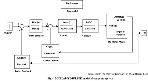
The complete simulation model is built in SIMULINK and shown in Fig.4.

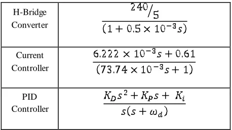
Table 3 lists the transfer functions of the different blocks in the model.

Table 3: Transfer function of different blocks

M otor

where

Current Sensor

Tacho

Generator

+

-

+

-

Den(s)

Num(s)

73.74e-3s+1

240/5

0.5e-3s+1

5/523

0.80e-3s+1

Armature Current

Voltage

Angular

Velocity W

5/183.26

25e-3s+1 Angular

Velocity PID Controller Current

Controller

H-Bridge Converter

DC Motor Model

Current Sensor

Techo Feedback

Continuous

Power Gui

H-Bridge Converter

Current Controller

PID Controller

5

RESULTS

Fitness function in the GA function is configured to optimize different types of errors. These errors are the return values from fitness function. The Genetic Algorithm uses this return value as the fitness parameter to evaluate the individuals in the population and hence select the best candidates.

Different optimization functions and the resulting PID controller transfer function is listed below. Result for M otor Speed optimization for Absolute Error can be seen in Fig 8.The results for PID and GA parameters for different error models are complied in Table 4. The resulting time domain response is shown in Fig 5-9.

5.1

ITSE (Integral Time Square Error)

for i=1: length (velocity)

temp = (183.26/5)*command;

f=f + abs ((temp-velocity (i) ^2)*tout (i));

end

5.2

ITAE (Integral Time Absolute Error)

for i=1: length (velocity)

temp = (183.26/5)*command;

f=f +abs (temp- velocity (i))*tout (i);

end

5.3

Peak Overshoot

f = max (velocity);

5.4

Absolute Error

f = abs ((max (velocity)-183.26/5*command))

5.5

Squared Error

for i=1: length (simout)

temp = (183.26/5)*command;

f=f+ (temp-simout (i)) ^2;

end

Table 4: Optimized PID parameters

Parameter Kp Ki Kd ωd Generations

ITSE 62

ITAE 9.917 7.689 3.804 2.019 67

Peak Overshoot

9.039 3.734 8.223 3.086 51

Abs Error 8.883 1.642 7.605 3.117 24

Squared Error

Fig 5: Motor S peed optimized for ITS E

Fig 6: Motor S peed optimized for ITAE

Fig 7: Motor S peed optimized for Peak Overshoot

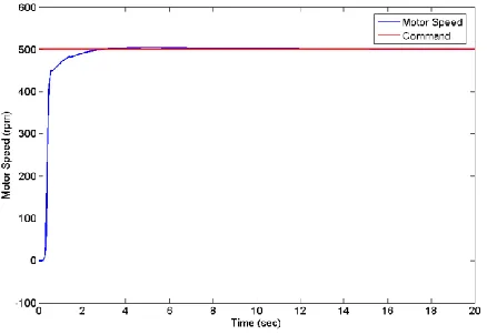
Fig 8: Motor S peed optimized for Absolute Error

Fig 9: Motor S peed optimized for S quared Error

6. CONCLUSON & FUTURE WORK

Parallel form PID which is also known as non- interacting form and GA parameters are obtained for different error models. It is observed that the optimization for absolute error results in the minimum deviation of the output from the commanded input velocity. However the time taken to reach the desired value is higher. Optimization for ITAE on the other hand gives a fast response as well as minimum steady state error but at the cost of increased overshoot. Other optimizations give nearly similar results. Hence, it is inferred that optimization for ITAE gives the best system performance if the overshoot can be accommodated.

7.

ACKNOWLEDGMENTS

The authors would like to express their cordial thanks to M r. Ashutosh Kumar and M r. Kashyap Dhruve of Planet-i Technologies for their much valued support and advice.

8. REFRENCES

[1] Boldea and S.A. Nasar. Linear electric actuators and generators. Cambridge university press,1997

[2] E. Cerruto, A. Consoli, A. Raciti, and A. Testa. A robust adaptive controller for PM motor drives in robotic applications. Power Electronics, IEEE Transactions on, 10(1):62–71, 1995.

[3] N. Hemati, J.S. Thorp, and M .C. Leu. Robust nonlinear control of brushless DC motors for direct drive robotic applications. Industrial Electronics, IEEE Transactions on, 37(6):460–468, 1990.

[4] PM Pelczewski and U.H. Kunz. The optimal control of a constrained drive system with brushless dc motor. Industrial Electronics, IEEE Transactions on, 37(5):342– 348, 1990.

[5] D.E. Goldberg. Genetic algorithms in search, optimization, and machine learning. Addison-wesley,1989.

[6] K. Kristinsson and G.A. Dumont. System identification and control using genetic algorithms. Systems, M an and

Cybernetics, IEEE Transactions on, 22(5):1033–1046, 1992.

[7] C. Vlachos, D. Williams, and JB Gomm. Genetic approach to decentralised PI controller tuning for multivariable processes. In Control Theory and Applications, IEEE Proceedings-, volume 146, pages 58–64. IET, 1999.

[8] Z. M ichalewicz, C.Z. Janikow, and J.B. Krawczyk. A modified genetic algorithm for optimal control problems. Computers & M athematics with Applications,23(12):83– 94, 1992

[9] BL Thereja. A Text Book of Electrical Technology, Volume II. S Chand & Co, New Delhi, 1992

[10]P. Pillay and R. Krishnan. M odeling, simulation, and analysis of permanent-magnet motor drives. II. The brushless DC motor drive. Industry Applications, IEEE Transactions on, 25(2):274–279, 1989

[11]D.G. Holmes, T.A. Lipo, and TA Lipo. Pulse width modulation for power converters: principles and practice. Wiley-IEEE Press, 2003.

[12]L. Chambers. Practical handbook of genetic algorithms: complex coding systems. CRC, 1999.