Optimized Power Schemes for Wireless Sensor
Network by using Threshold Techniques
Uma Sharma
I.T Department, R.K.G.I.T.W Ghaziabad U.P, India
Pushpa
I.T Department, Accurate Institute of Tech. & Mgmt. Gr. Noida, U.P, India
ABSTRACT
One of the main design issues for a sensor network is conservation of the energy available at each sensor node. Optimal routing tries to maximize the duration over which the sensing task can be performed, but requires historical knowledge. This paper proposes packet profile based (PPB) scheme with certain threshold value to increase the battery power of sensor node. Profile based scheme is based on probability of past information of packet transfer, and save this information as a small data base of each node. Reliability of this scheme is rely on life time of most probabilistic node .This study also compares the result with flooding scheme and PPB without threshold value.Simulation results show that the better energy consumption is achieved by the proposed scheme when compared to the conventional techniques.
Keywords
Wireless Sensor Network, flooding, profile based, power efficient, threshold.
1. INTRODUCTION
Nowadays, Wireless Sensor Networks (WSN) has become a very significant new field in wireless technology. As evident, the wireless sensor networks are comprised of thousands of inexpensive sensor nodes. The sensor node consists of processing capability, memory, RF transceiver, power source and accommodates various sensors [4, 9]. Sensor nodes sense the event that occurs in the network and then pass the packets to the sink following a path. For a WSN to meet real world requirements, it has to be reliable, power efficient, and time efficient. Possible applications of sensor networks are of interest to the most diverse fields. Environmental monitoring, warfare, child education, surveillance, micro-surgery, and agriculture are only a few examples [10]. All these application mainly include the sensor node which are capable of data gathering, processing, transmitting and storing information. In a WSN application, all sensor nodes can transmit and receive the packet. These nodes periodically transmit data to single sink node which is based on many to one communication model. As due to higher bit rate in the downstream direction, the congestion appears at the node. This Congestion leads to large number of dropping of packets and increases in transmission latency and consequently affects energy efficiency. So it must be handled efficiently. There can be two types of congestion in WSN: link level and node level congestion. Thus, the protocol is chosen, collisions could occur when multiple active sensor nodes try to seize the channel at the same time. This increases packet service time and decreases both link utilization and overall throughput. This causes the wastage of energy at sensor nodes. Both node level and link level congestion have great impact on energy efficiency and QOS.
In wireless sensor network, there are so Node level congestion is very common in traditional networks and it is due to the buffer overflow in the node which leads to the packet loss and
increases queuing latency. Packet loss leads to retransmission and requires more energy [1].
In link level congestion, as the wireless channel is shared by several nodes, if CSMA many challenges[5-7]. The main challenges are how to enhance lifetime of a node thus automatically enhancing lifetime of network and how to provide reliable communication to network. Since sensor network totally rely on battery power, the main aim for enhancing lifetime of network is to conserve battery power or energy with some security considerations.
This paper is organized as follows. Section II presents related work. In Section III, the proposed scheme on the basis of packet transmission weightage factor by reducing number of packet dropping probability using the threshold value is discussed. Section IV represents the simulation, results and its performance analysis. Finally section V concludes the paper.
2. RELATED WORK
2.1 Flooding
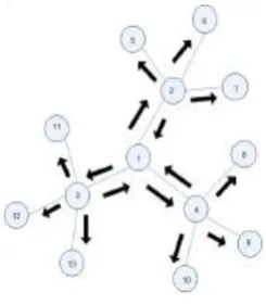
[image:1.595.372.495.484.625.2]The conventional mechanism for relaying data from individual sensors to base station is Flooding or Gossiping [12]. Flooding occurs when each sensor on receiving a data packet broadcasts the same to its every neighbor. This process continues until it reached at the destination or the maximum number of hops for the packet is reached.
Fig 1: Broadcasting of packets
Due to the flooding raises broadcast storms which are become unmanageable as shown in Fig 1.
redundancies, contentions and collisions. These problems result in wasteful consumption of node energies. Due to the broadcast storm sensor nodes are not able to afford these problems because each node has only limited energy reserves in the form of small batteries. Designing of routing protocols in WSNs using flooding approach does not seem to be an appropriate approach due to above defined problems associated with flooding.
Disadvantage of using flood based scheme
1. Node has to broadcast packet to all the node of neighboring list in range.
2. The entire receiving packet node has to again find out neighboring node & broadcast the packet to the entire node until the sink node. Finally, power of each packet will be reduced.
3. Nodes redundantly receive multiple copies of the same data message and implosion is detected. Then, as the event may be detected by several nodes in the affected area, multiple data messages containing similar information are introduced into the network.
4. Number of hop can be increased.
5. Time of successful packet transmission can be increased and subsequently rate of packet loss will be increased.[2]
2.2 Proposed Packet Profile Based (PPB)
Scheme
To overcome limitation of flooding this study is proposing a new scheme based on packet transfer analysis. Suppose there are wireless sensor network with 15 nodes and historical information about the reliable packet broadcasting and successful delivery of packets to the sink node is as follows: [3,11]. 1/2/1/2/1/7/1/7/1/7/8/1/8/1/8/1/8/1/8/1/8/1/9/1/9/2/3/2/3/2/7/2/8/ 2/8/2/8/2/8/2/8/2/8/2/8/2/8/2/9/2/9/2/9/2/9/2/9/2/9/3/4/3/4/3/8/3/ 8/3/8/3/8/3/8/3/8/3/8/3/8/3/9/3/9/3/9/3/9/3/9/3/9/3/9/3/9/3/9/3/10 /3/10/3/10/4/3/4/5/4/5/4/9/4/9/4/9/4/9/4/9/4/9/4/9/4/9/4/10/4/10/ 4/10/4/10/4/10/4/11/4/11/4/11/5/6/5/6/5/10/5/10/5/10/5/10/5/10/ 5/11/5/11/5/11/5/11/6/5/6/11/6/11/6/11/6/11/7/2/7/8/7/8/7/8/7/8/ 7/12/7/12/7/12/7/12/7/12/7/12…
Now build a probability transition matrix (S) to most likelihood transition. X X X X X X X X X X X X X X X X X X X X X X X X X X X X X X X X X X X X X X X X X X X X X X X X X X X X X X X X X X X X X X X X X X X X X X X X X X X X X X X X X X X X X X X X X X X X X X X X X X X X X X X X X X X X X X X X X X X X X X X X X X X X X X X X X X X X X X X X X X X X X X X X X X X X X X X X X X X S 2 2 3 4 1 6 3 5 1 3 6 1 1 3 6 1 1 1 2 2 7 2 2 2 1 3 2 5 1 2 2 1 1 3 4 8 2 5 2 3 2 6 6 2 2 4 3 4 5 2 2 3 5 8 2 2 3 8 8 2 2 6 8 1 2 2 2 6 3 2
By adding all the column of S, get maximum transition state (MTS) in following row vector MTS.
MTS=[7,11,11,8,8,3,11,45,39,23,13,20,10,11,18]
According MTS row vector node I is most probabilistic node as it has maximum transition state 45 and so on.
Now make following assumptions about this system modeling:-
Let each node is one meter far away from each other.
Node can be in range if they are one meter or sqrt (2).
Each node has small data base of maximum transition observed from history.
Each node has 100 unit of power.
Each node that will process the packet, their power will be reduced by 1unit.
Each node is taking 1ms to transfer one packet to another node.
Let node C sense the data packet then it will check the list of neighboring node which are in range. If any node is not as sink node then check its data base that which node has highest probability of transition and also available in list of neighboring node. If sink node is available in the list then transfer the packet directly to the sink node. For example node I has highest probability of transition and it is also available in the list of neighboring node of C. Also rather then broadcast the packet to the entire neighboring node, packet is only transfer to node I. node I will perform same way until it achieve the sink node.
Algorithm:
(i) Assign 100 unit to each sensor node. (ii) Assign Maximum number of packets in Pmax (iii) Node sense the packet.
(iv) Find out the neighboring list of node [all node which are 1m or sqrt (2) m away from each other will be consider as member of neighbor list]
(v) Check sink node in neighboring list:
(vi) Else search in data base in ascending order which has highest transition probability in vector MTS and also available in the list of neighboring node.
(vii) If search==true then transfer the packet to that node. And also hop=hop+1, power=power-1 for receiving node.
(viii) Else transfer the packet to any node available in neighboring list. And also hop=hop+1, power=power-1 for receiving node.
(ix) Go to step-(iv) (x) End
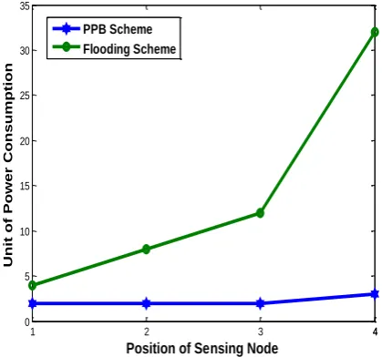
The above algorithm performs well compared to flooding algorithm. Figure (2) shows the comparison of the graph between the packet profile based technique and the flood based system. Finally, It shows that power consumed by using PPB scheme is much less as compared to the flood based scheme.
1 2 3 44
0 5 10 15 20 25 30 35
Position of Sensing Node
Unit
of Pow
er C
onsumpt
ion
PPB Scheme Flooding Scheme
Fig. 2: Comparison graph for power Optimization
According MTS row vector the most probabilistic node is H, which is used to transfer the packet to another node especially sink node as sink node is neighbor of node H. PPB scheme provide following advantages:
1. Less number of hops.
2. Increase reliability of packet.
3. Reduces number of packet failure.
4. Less power consumption
Efficiency and reliability of PPB scheme rely on life time of most probabilistic node such as H, I etc. But by this scheme most probabilistic node will become overloaded and congested and also life time of this node will depreciated very fast hence after some time this node will be no longer available. To overcome this problem we are using the concept of threshold value.
3. PPB WITH THRESHOLD TECHNIQUE
The environment consists of 15 nodes uniformly distributed over a space. In Simulation network, every two nodes are 1m or sqrt(2) apart from each other. [image:3.595.68.278.284.480.2]The node attributes are chosen according to the proposed algorithm to store the power of node, the maximum transition state (MTS) and the number of packets, the node can have in queue for processing. The simulation assumes the base station to be fixed at the origin and is a powerful node.
Fig 3: Node Placement
The plot in Fig. 3 shows the distribution of the nodes. The positions of all the nodes are evenly distributed. The id of the node is written alongside the circle. Networks are in layered form. First Layer from node A to F is acting as a sensor node. Second layer from G to K and M to N are transmitting the packet. Node L is sink node.
Here we consider that each node can process certain number of packet Pmax. If power of most probabilistic node become 80 % and number of packet get exceeded from Pmax then next incoming packet is transferred on other next most probabilistic node.
Here we proposed algorithm with threshold techniques:
(i) Assign 100 unit to each sensor node. (ii) Assign no. of packets to Pmax (iii) Enter the threshold value (Thvalue). (iv) Node sense the packet.
(v) If power<= Thvalue then transfer the packet to next most probabilistic node.
(vi) Find out the neighboring list of node [all node which are 1m or sqrt (2) m away from each other will be consider as member of neighbor list] (vii) Check sink node in neighboring list:
If sink node is available in neighboring list send the packet directly to the sink node, do hop=hop+1, power=power-1 for that node and go to step-(ix).
(viii) Else search in data base in ascending order which has highest transition probability in vector MTS and also available in the list of neighboring node. (ix) If search==true then transfer the packet to that
node. And also do hop=hop+1 and power=power-1 for receiving node.
(x) Else transfer the packet to any node available in neighboring list. And also hop=hop+1, A
B C D E
G H I J
L M N
K
F
(xi) Go to step-(iv) (xi) End
PPB scheme with threshold value perform well compare to PPB scheme without threshold value. In next paragraph we evaluated performance of purposed scheme.
4. PERFORMANCE EVALUATION
To assess the performance of PPB with threshold, we simulated its performance using C and compared its probabilistic performance with different value of Thvalue.
one of the major objective of this work has been to improve the lifetime of the sensor networks. So we compare the lifetime in the proposed methodology with the existing protocols. Typically, there are three different measures for the lifetime of a WSN, namely,
1. The time till the most probabilistic node exhaust its energy with different threshold values.
2. The time till the last node exhaust its energy with reliability.
The Figure 4 shows the lifetime of Hth node by using PPB with Threshold w.r .to different size of packets
0.0 10.0 20.0 30.0 40.0 50.0 60.0 70.0
80 75 70 65 0
Thresh hold values (Thvalue)
L
ife
ti
m
e
p
r
o
b
a
b
il
ity
o
f
H
th
node
Pmax=1 Pmax=3 Pmax=5
Life time of H th node w.r.to different size of packet
Fig. 4 Life time of Hth node by using PPB with Threshold w.r.to different size of packets
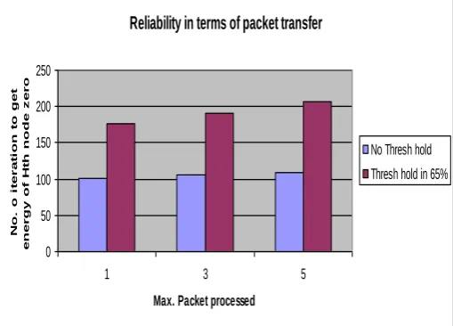
Reliability can be measured in terms of:
1) Number of iterations in terms of number of packet
transfer as shown in figure 5
2) Percentage of lifetime with respect to the Hth node as
shown in figure 6
Thus, the simulation is transferring reliable number of packets without any loss of packets and the reliability is shown in the graph in terms of number of successful packet transfer iterations. The analysis also shows that the lifetime has been increased from 32% to 61% in case of maximum number of packets delivered by a node
Reliability in terms of packet transfer
0 50 100 150 200 250
1 3 5
Max. Packet processed
N
o.
o
i
t
e
r
a
t
i
on
t
o
ge
t
e
ne
r
gy
of
H
t
h
no
de
z
e
r
o
No Thresh hold
[image:4.595.311.566.76.259.2]Thresh hold in 65%
Fig. 5. Reliability in terms of Packet Transfer by Hth node
Comparison of percentage of lifetime w.r.to the H
thnode
0 10 20 30 40 50 60 70
1 3 5
Maximum Packets
%
of
Li
f
e
t
i
m
e
of
H
th
no
de
No thresh hold value
[image:4.595.310.549.300.482.2]Thresh hold value
Fig .6 Comparison of percentage of lifetime of Hth node
Thus, the proposed PPB algorithm with PPB increases the lifetime of node and so, as it increases the lifetime of node, it will also increase the network lifetime.
5. CONCLUSIONS
6. REFERENCES
[1] V. Vijaya Raja, R. Rani Hemamalini and A. Jose Anand, “ Study of Traditional Fairness Congestion Control Algorithm in Realistic WSN Scenarios”, International Journal of Engineering Research and Applications (IJERA), ISSN: 2248-9622, Vol. 1, Issue 4, pp.1645-1651.
[2] Luis Javier García Villalba, Ana Lucila Sandoval Orozco, Alicia Triviño Cabrera and Cláudia Jacy Barenco Abbas, “Routing Protocols in Wireless Sensor Networks”, Sensors 2009, 9, 8399-8421; doi:10.3390/s91108399
[3] Pushpa, Amit Sehgal, Rajeev Agarwal, “New Handover Scheme Based on User Profile: A Comparative Study”, Communication Software and Networks, 2010. ICCSN '10, Issue Date: 26-28 Feb. 2010, pp 18 - 21, E-ISBN: 978-1-4244-5727-4 ,Print ISBN: 978-1-4244-5726-7 ,doi: 10.1109/ICCSN.2010.102
[4] I. Akyildiz, W. Su, Y. Sankarasubramaniam, and E. Cayirci, "A survey on sensor networks," IEEE Communications Magazine, Volume: 40 Issue: 8, pp.102-114, August 2002.
[5] A. Hac, ”Wireless Sensor Network Design”, New York: Wiley, 2003.
[6] P. Santi, “Topology Control in Wireless Ad Hoc and Sensor Networks”, Chichester: Wiley, 2005.
[7] P. Kwaśniewski and E. Niewiadomska-Szynkiewicz, “Optimization and control problems in wireless ad hoc networks”, Evolutionary Computation and Global Optimization. Warsaw: WUT Publ. House, 2007, No. 160, pp. 175–184.
[8] Seada, K.; Zuniga, M.; Helmy, A.; Krishnamachari, B. ,”Energy-Efficient Forwarding Strategies for Geographic Routing in Lossy Wireless Sensor Networks”, Proceedings of the Second International Conference on Embedded Networked Sensor Systems, Baltimore, MD, USA, November, 2004; pp. 108–121.
[9] S. Tilak, N. Abu-Ghazaleh, W. Heinzelman,” A taxonomy of wireless micro-sensor network models", ACM SIGMOBILE Mobile Computing and Communications Review, Volume 6, Issue 2 (April 2002), pp. 28-36.
[10]J. Hill, System Architecture for Wireless Sensor Networks. Ph.D.thesis, University of California at Berkeley, Spring 2003.
[11]Uma Sharma,, Pushpa “ Power Optimization Techniques in Wireless Sensor Network by using Packet Profile based Scheme” IJCSI International Journal of Computer Science Issues, Vol. 9, Issue 3, No 3, May 2012 ISSN (Online): 1694-0814.