Impulsive Synchronization of Hyperchaotic Lü Systems with Two Methods

http://dx.doi.org/10.4236/ijmnta.2015.41001

Impulsive Synchronization of Hyperchaotic

Lü Systems with Two Methods

Mingjun Wang

School of Information Engineering, Dalian University, Dalian, China Email: [email protected]

Received 15 January 2015; accepted 11 February 2015; published 16 February 2015

Copyright © 2015 by author and Scientific Research Publishing Inc.

This work is licensed under the Creative Commons Attribution International License (CC BY). http://creativecommons.org/licenses/by/4.0/

Abstract

In the paper, impulsive synchronization of two hyperchaotic Lü systems with different initial con-ditions is studied. The sufficient concon-ditions on feedback strength and impulsive distances are es-tablished from two different angles to guarantee the synchronization. The relevant theoretical proofs are presented. Numerical simulations show the effectiveness of the methods.

Keywords

Impulsive Synchronization, Impulsive Distance, Hyperchaotic Lü System, Largest Lyapunov Exponent

1. Introduction

hyper-chaotic Lü system is studied. Based on the boundedness and the largest Lyapunov exponent, two different suffi-cient conditions are established to guarantee the synchronization. These two methods are analyzed and com-pared. Numerical simulations show the effectiveness of these methods.

2. Impulsive Synchronization Theory

Suppose a n-dimensional chaotic system as

(

,

)

F t

=

X X (1) choose system (1) as drive system, response system is as follows

( )

(

)

( ) ( ) ( )

( )

(

)

( )

0

( )

,

, 1, 2, 3,

0 i

i i i i i

F t t t

t t t t t t i

t

+ − +

+

 = ≠



 _{= − = − = = =}

 

= 

Y Y

Y Y Y Y Y BE Y Y



  (2)

B is a matrix which stands for a linear combination of Y−X, let B=diag

(

b b₁, ₂,,bn

)

; The error vector is E=Y−X; t_i is the discrete time at which the impulse is transmitted. According to system (1) and system (2), we can get the error system

( )

(

)(

)

(

)

, , _i

i

F t F t t t

t t

 _{− ≠}

 

= =



=

Y X

E BE

E





(3)

Suppose the impulsive distance

η

is invariable, η=t_i+₁−t_i, if we can obtain lim

( )

0

t→∞ E t = under some- conditions, system (1) and system (2) can be synchronized by impulses. Next we will take hyperchaotic Lü sys-tem as example for detailed description.

3. Implement of Impulsive Synchronization

3.1. Description of Hyperchaotic Lü System

Hyperchaotic Lü system [17] is described as

(

)

x a y x w

y xz cy

z xy bz

w xz dw

 = − +



= − + 



= −

  = + 

   

(4)

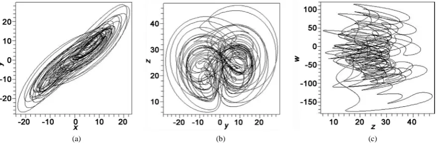
in this paper choose a=36, b=3, c=20 and d=1 _{so that system (4) exhibits a hyperchaotic behavior} [17], Figure 1 shows the projections of hyperchaotic Lü system’s attractor.

[image:2.595.96.538.560.707.2]

(a) (b) (c)

Choose hyperchaotic Lü system

(

)

1 2 1 4

2 1 3 2

3 1 2 3

4 1 3 4

x a x x x

x x x cx

x x x bx

x x x dx

= − +   = − +   = −   = +      (5)

as drive system. System (5) can be described as

( )

ϕ

=

X AX + X (6)

where

( )

1 3

1 2

1 3

0

0 1

0 0 0

, .

0 0 0

0 0 0

a a x x c x x b x x d

ϕ

−         ₋     =_{ } =_{ } −         A X

The response system is described as

( )

(

)

( ) ( ) ( )

( )

(

)

( )

0

( )

, 1, 2, 3,

, 1, 2, 3,

0

i

i i i i i

t t i

t t t t t t i

t

ϕ

+ − + +  = ≠ =   _{= − = − = = =}   = 

Y AY + Y

Y Y Y Y Y BE Y Y

 _

  (7)

where

[

]

[

] [

]

(

)

T 1 2 3 4

T T

1 2 3 4 1 1 2 2 3 3 4 4

1 2 3 4

, , , ,

, , , , , , ,

diag , , , .

y y y y

e e e e y x y x y x y x

b b b b

= = = − − − − = Y E B .

The error system is

(

) (

)

(

)

i i t t t t ρ  = + ≠   = = 

E AE X,Y

E BE 

 (8)

where

(

)

( ) ( )

1 3 1 3 3 1 1 3

1 2 1 2 2 1 1 2

1 3 1 3 3 1 1 3

0 0

, x x y y y e x e

y y x x y e x e

y y x x y e x e

ρ

ϕ

ϕ

     ₋  _{− −}      = − =_{  }= _ − +  ₋   ₊     

X Y Y X .

Next the sufficient conditions on feedback strength and impulsive distances will be established from two dif-ferent angles to guarantee the synchronization.

3.2. Based on the Boundedness of Chaotic System

Theorem 1 Suppose M≥max

(

y₁, y₂, y₃

)

,

β

is the largest eigenvalue of

(

I+B

) (

T I+B

)

(

)

(

I=diag 1,1,1,1

)

,

λ

is the largest eigenvalue of 0.5

(

A+AT

)

, the constant

ε

>1,

η

is impulsive dis-tance, if choose suitable

β

and

η

such that

( ) (

)

ln εβ + 2λ+3M η≤0, (9)

then system (6) and system (7) can be synchronized.

Proof: Choose Lyapunov function as

T

0.5

(

)

(

)

(

(

)

)

(

)

(

)

(

)

(

)

T _T T T

3 1 2 2 1 3 3 1 4 1 3 4

1 2 1 3 1 4 3 4

1 2 1 3 1 4 3 4 2 3 2 4

0.5 , 0.5 ,

0.5

2 2

2 3 2 3 .

V

y e e y e e y e e x e e

V M e e e e e e e e

V M e e e e e e e e e e e e

V MV M V

ρ ρ λ λ λ λ = = − + + + ≤ + + + + ≤ + + + + + + ≤ + = +

AE + X Y E + E AE + X Y E A + A E



(11)

When t∈

(

ti−₁,ti

]

(

i=1, 2, 3,

)

, we have

( )

(

)

(

( )

)

(2 3 )( 1)

1 e

i

M t t i

V t V t+ λ+ −−

−

≤

E E . (12)

When t=t_i, system (8) is a discrete system, according to Equation (8), we get

( )

(

)

(

) ( ) (

T

) ( )

( ) ( )

T

(

( )

)

0.5 0.5

i i i i i i

V E t+ = _ I+B E t _ I+B E t ≤ βE t E t =βV E t (13)

Let i=1, according to Equation (12), when t∈

(

t t₀,₁

]

,

( )

(

)

(

( )

)

(2 3 )( 0)

0 e

M t t

V E t ≤V E t+ λ + − (14) When t=t₁, we obtain

( )

(

)

(

( )

)

(2 3 )(1 0)

1 0 e

M t t

V E t ≤V E t+ λ + − (15) From Equation (13) and Equation (15),

( )

(

)

(

( )

)

(

( )

)

(2 3 )(1 0)

1 1 0 e

M t t

V E t+ ≤βV E t ≤βV E t+ λ+ − (16) According to Equation (12), when t∈

(

t t₁, ₂

]

,

( )

(

)

(

( )

)

(2 3 )( 1)

(

( )

)

(2 3 )(1 0) (2 3 )( 1)

(

( )

)

(2 3 )( 0)

1 e 0 e e 0 e

M t t M t t

M t t M t t

V E t ≤V E t+ λ+ − ≤βV E t+ λ+ − λ+ − =βV E t+ λ+ − (17) In the same way, when t∈

(

ti−₁,ti

]

(

i=1, 2, 3,

)

,

( )

(

)

1

(

( )

)

(2 3 )( 0)

0 e

M t t i

V E t ≤β−V E t+ λ+ − (18) From Equation (9), yield

(2 3 ) e λ Mη 1

εβ

+ _≤

(19)

hence

( )

(

)

( )( )

1

1 1 2 3 1 2 3 1 1 1 e e i

i i M i

M

i λ η λ η

β ε ε − − − + − + −

≤ = (20)

Substitute Equation (20) into Equation (18), we can obtain when t∈

(

ti−₁,ti

]

(

i=1, 2, 3,

)

,

( )

(

)

1 (2 3 )( )1

(

( )

0

)

(2 3 )( 0) 1

(

( )

0

)

(2 3 )( 1)

1 1

e e

e

i

M t t M t t

i M i

i

V t _{λ η}V t λ V t λ

ε ε − + − + − + + − + − − ≤ =

E E E (21)

Since t∈

(

ti−₁,ti

]

, t−ti−1≤η．From the assumption given in Theorem 1, we have lim

(

( )

)

0

i→∞V E t = , Thus obtain lim

( )

0

t→∞ E t = , i.e. system (6) and system (7) will be synchronized when Equation (9) is satisfied.

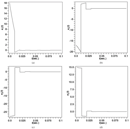
In this numerical simulation, let B=diag

(

−1.1, 1.1, 1.1, 1.1− − −

)

, impulsive distance η =0.01 sec.

( )

. A time step of size 0.0001(sec.) is employed and fourth-order Runge-Kutta method is used to solve Equation (6) and Equation (7). The initial states of the drive system (6) and the response system (7) are taken as X

( ) (

0 = −10, 5,8,15

)

and Y

( ) (

0 = 8, 12, 20, 30− −

)

. The error system (8) has the initial state E

( ) (

0 = 18, 17, 28,15− −

)

. Figure 2 shows the history of e t₁

( )

, e t₂

( )

, e t₃

( )

, e t₄

( )

in the error system (8). From Figure 2, we can see that

( )

1

e t , e t₂

( )

, e t₃

( )

, e t₄

( )

are steady near zero at last, i.e., system (6) and system (7) can be synchronized when B=diag

(

−1.1, 1.1, 1.1, 1.1− − −

)

and η =0.01 sec.

( )

.

3.3. Based on the Largest Lyapunov Exponent of Chaotic System

Theorem 1 provides sufficient condition for the synchronization of system (6) and system (7), but Equation (9) is not necessary condition. Through simulations we find that the above condition is too rigorous. In fact the qualified impulsive distance can be much larger than

η

solved from Equation (9). Next we will present a new condition based on the largest Lyapunov exponent, which is much looser than Equation (9).

(a) (b)

[image:5.595.89.512.279.698.2]

(c) (d)

Suppose the initial distance between system (6) and system (7) is E

( )

0 , the largest Lyapunov exponent of

system(6) is λ₁. Without control, the largest distance between system (6) and system (7) will not go beyond

( )

1

0 λ t

E  after a short time t (considering the average case). Generally speaking, the longest predicted time of the chaotic system is 1λ₁ [18]. Based on the above theory, we can obtain the following conclusions.

Theorem 2 Suppose

β

is the largest eigenvalue of

(

I+B

) (

T I+B

)

(

I=diag 1,1,

(

,1,1

)

)

, λ₁ is the largest Lyapunov exponent of system (6), the constant

ε

>1,

η

is impulsive distance. Let η<1λ, if choose suitable

β

and

η

such that

1

lnεβ+2λη≤0, (22) System (6) and system (7) can be synchronized

Proof: Suppose

( )

( ) ( )

T

V t =E t E t , (23)

then

( )

( )

( ) ( )

T

0 0 0 0

V t =V t+ =E t E t , (24) hence

( )

( ) ( )

T 1

( )

T 1

( )

21

( )

1 1 1 e 0 e 0 e 0

V t =E t E t ≤_ λ ηE t  _{ } λ ηE t _= λ ηV t , (25)

( )

(

) ( ) (

T

) ( )

( ) ( )

T

( )

21

( )

1 1 1 1 1 1 e 0

V t+ =_ I+B E t _ I+B E t ≤βE t E t =βV t ≤β λ ηV t . (26)

( )

( ) ( )

1

( )

1

( )

1

( )

1 1

( )

T

T 2 2 2

2 2 2 e 1 e 1 e 1 e e 0

V t =E t E t ≤_ λ ηE t+ _{ }  λ ηE t+ _= λ ηV t+ ≤β λ η λ ηV t , (27)

( )

(

) ( ) (

T

) ( )

( ) ( )

T

( )

(

21

)

2

( )

2 2 2 2 2 2 e 0

V t+ =_ I+B E t _ I+B E t ≤βE t E t =βV t ≤ β λ η V t . (28) In the same way, we have

( )

(

21

)

( ) (

)

0

e i 1, 2, 3,

i

V t+ ≤ β λ η V t i=  , (29)

According to the condition of Theorem 2: lnεβ+2λη₁ ≤0, we have

1

2

eλ η 1 1

β ≤ ε< , (30)

According to Equation (29) and Equation (30), we obtain lim

( )

i 0 i V t

+

→∞ = , then limt→∞ E

( )

t =0, i.e. system (6) and system (7) can be synchronized if the condition of Theorem 2 is satisfied.

Here, we still choose a=36, b=3, c=20, d=1 _{so that system (5) exhibits hyperchaotic behavior} [17]. For this system, the largest Lyapunov exponent λ =₁ 1.065. Suppose system (5) is described as system (6), choose system (6) as drive system, system (7) is the relevant response system, system (8) is the error system, we

have X =

[

x x x x₁, ₂, ₃, ₄

]

T, Y =

[

y y y y₁, ₂, ₃, ₄

]

T, E=

[

e e e e₁, ₂, ₃, ₄

] [

T = y₁−x y₁, ₂−x y₂, ₃−x y₃, ₄−x₄

]

T. Choose

(

)

diag 1.1, 1.1, 1.1, 1.1

= − − − −

B ,

ε

=5, substitute them into Equation (22), we obtain

η

≤1.406. Considering 1

1 0.939

η< λ = , we have the following results: when B=diag

(

−1.1, 1.1, 1.1, 1.1− − −

)

,

η

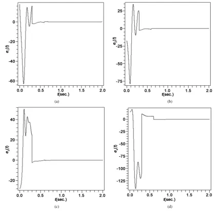
<0.939, system (6) and system (7) can achieve impulsive synchronization.

In this numerical simulation, let B=diag

(

−1.1, 1.1, 1.1, 1.1− − −

)

, impulsive distance η =0.3 sec.

(

)

. A time step of size 0.0001(sec.) is employed and fourth-order Runge-Kutta method is used to solve Equation (6) and Equation (7). The initial states of the drive system (6) and the response system (7) are taken as X

( ) (

0 = −10, 5,8,15

)

and Y

( ) (

0 = 8, 12, 20, 30− −

)

. The error system (8) has the initial state E

( ) (

0 = 18, 17, 28,15− −

)

. Figure 3 shows the history of e t₁

( )

, e t₂

( )

, e t₃

( )

, e t₄

( )

in the error system (8). From Figure 3, we can see that

( )

1

(a) (b)

(c) (d)

Figure 3. (Based on the largest Lyapunov exponent) Synchronization error system (8) states: e t₁

( )

, e t₂

( )

,

( )

3

e t , e t₄

( )

.

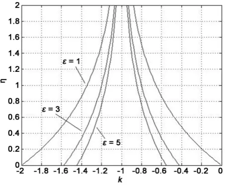
3.4. Comparison of Two Methods

If system (6) and system (7) achieve synchronization, system (8) will be steady at zero. Suppose B=diag

(

k k k k, , ,

)

,

η

stands for impulsive distance, Figure 4 shows the boundaries of the stable region for Theorem 1, Figure 5 shows the boundaries of the stable region for Theorem 2. (Taking ε=1, 3, 5 as examples, the region below the boundary is stable, not considering η<1λ₁ in Figure 5).

From Figure 4 and Figure 5, we can see that the requirement of impulsive distance in Theorem 1 is more ri-gorous than Theorem 2. Comparing the methods of Theorem 1 and Theorem 2, the former is based on the boundedness of chaotic system, it considers the extreme case all the time, while the latter is based on the largest Lyapunov exponent of chaotic system, it represents the average case. Therefore, the sufficient condition in Theorem 1 is a very small part of the condition in Theorem 2. Of course, in view of the requirements of syn-chronous time and quality, it is not suitable to choose very large impulsive distance in practical applications.

4. Conclusion

[image:7.595.86.522.82.495.2]

[image:8.595.187.412.85.265.2]

Figure 4. The boundaries of the stable region for Theorem 1.

Figure 5.The boundaries of the stable region for Theorem 2.

the sufficient conditions for synchronization and relevant analysis and comparison are presented. Mohammad et al. adopted the first method to study impulsive synchronization of hyperchaotic Chen systems [19]. The second method has not been reported before. Obviously it is more compatible than the first one. Numerical simulations show the effectiveness of the methods.

Acknowledgements

The work was supported by Doctor Specific Funds of Dalian University.

References

[1] Pecora, L. and Carroll, T. (1990) Synchronization in Chaotic Systems. Physical Review Letters, 64, 821-824.

http://dx.doi.org/10.1103/PhysRevLett.64.821

[2] Carroll, T. and Pecora, L. (1991) Synchronizing Chaotic Circuits. IEEE Transactions on Circuits Systems, 38, 453-456.

http://dx.doi.org/10.1109/31.75404

[3] Chen, G. and Dong, X. (1998) From Chaos to Order: Methodologies, Perspectives and Applications. World Scientific, Singapore.

[image:8.595.187.411.294.480.2]

[5] Wang, X.Y. (2003) Chaos in the Complex Nonlinearity System. Electronics Industry Press, Beijing.

[6] Chen, G.R. and Lü, J.H. (2003) Dynamical Analyses, Control and Synchronization of the Lorenz system family. Science Press, Beijing.

[7] Kemih, K., Bouraoui, H., Messadi, M. and Ghanes, M. (2013) Impulsive Control and Synchronization of a New 5D Hyperchaotic System. Acta Physica Polonica A, 123, 193-195. http://dx.doi.org/10.12693/APhysPolA.123.193

[8] Itoh, M., Yang, T. and Chua, L. (2001) Conditions for Impulsive Synchronization of Chaotic and Hyperchaotic Sys-tems. International Journal of Bifurcation and Chaos, 11, 551-560. http://dx.doi.org/10.1142/S0218127401002262

[9] Chai, X., Gan, Z. and Shi, C. (2013) Impulsive Synchronization and Adaptive-Impulsive Synchronization of a Novel Financial Hyperchaotic System. Mathematical Problems in Engineering, 2013, 751616.

http://dx.doi.org/10.1155/2013/751616

[10] Senouci, A. and Boukabou, A. (2014) Predictive Control and Synchronization of Chaotic and Hyperchaotic Systems Based on a T−S Fuzzy Model. Mathematics and Computers in Simulation, 105, 62-78.

http://dx.doi.org/10.1016/j.matcom.2014.05.007

[11] Candido, R. and Eisencraft, M. (2014) Channel Equalization for Synchronization of Chaotic Maps. Digital Signal Processing, 33, 42-49. http://dx.doi.org/10.1016/j.dsp.2014.07.001

[12] Xiao, X., Zhou, L. and Zhang, Z. (2014) Synchronization of Chaotic Lur’e Systems with Quantized Sampled-Data Controller. Communications in Nonlinear Science and Numerical Simulation, 19, 2039-2047.

http://dx.doi.org/10.1016/j.cnsns.2013.10.020

[13] Ren, Q. and Zhao, J. (2006) Impulsive Synchronization of Coupled Chaotic Systems via Adaptive-Feedback Approach.

Physics Letters A, 355, 342-347. http://dx.doi.org/10.1016/j.physleta.2006.02.053

[14] Chen, Y. and Guo, J. (2014) Synchronization of a Class of Chaotic Systems Using Small Impulsive Signal. Interna-tional Journal for Light and Electron Optics, 125, 6407-6412. http://dx.doi.org/10.1016/j.ijleo.2014.06.117

[15] Xi, H., Yu, S., Zhang, R. and Xu, L. (2014) Adaptive Impulsive Synchronization for a Class of Fractional-Order Chao-tic and HyperchaoChao-tic Systems. Optik—International Journal for Light and Electron Optics, 125, 2036-2040.

http://dx.doi.org/10.1016/j.ijleo.2013.12.002

[16] Xu, Y., Wang, Y. and Zhao, J. (2014) A New Chaotic System without Linear Term and Its Impulsive Synchronization.

Optik—International Journal for Light and Electron Optics, 125, 2526-2530.

http://dx.doi.org/10.1016/j.ijleo.2013.10.123

[17] Chen, A., Lu, J., Lü, J. and Yu, S. (2006) Generating Hyperchaotic Lü Attractor via State Feedback Control. Physica A:

Statistical Mechanics and its Applications, 364, 103-110. http://dx.doi.org/10.1016/j.physa.2005.09.039

[18] Lü, J., Lu, J. and Chen, S. (2002) Analysis and Applications of Chaotic Time Series. Wuhan University Press, Wuhan.

[19] Mohammad, H. and Mahsa, D. (2006) Impulsive Synchronization of Chen’s Hyperchaotic System. Physics Letters A,