Kinetic Foundation for the Multimoment Hydrodynamics Equations

http://dx.doi.org/10.4236/ojfd.2015.51010

Kinetic Foundation for the Multimoment

Hydrodynamics Equations

Igor V. Lebed

Zhukovsky Central Institute of Aerohydrodynamics, Moscow, Russia Email: [email protected]

Received 15 February 2015; accepted 4 March 2015; published 11 March 2015

Copyright © 2015 by authors and Scientific Research Publishing Inc.

This work is licensed under the Creative Commons Attribution International License (CC BY).

http://creativecommons.org/licenses/by/4.0/

Abstract

The equations for the pair distribution functions are derived directly from the second equation of the Bogolyubov-Born-Green-Kirkwood-Yvon (BBGKY) hierarchy. The derivation is fulfilled within the frameworks of the multiscale method. The equations for the pair distribution functions are the kinetic foundation for the multimoment hydrodynamics equations. Solutions to the equations for the pair distribution functions predetermine the possibility of constructing the hydrodynamics equations with an arbitrary number of principle hydrodynamic values specified beforehand. The tendency to increase the number of principal hydrodynamic values is caused by the necessity of interpreting the behavior of the system after the loss of stability. Solutions to the classic hydrody-namics equations constructed for only three principle hydrodynamic values are unable to predict the direction of instability evolution. Solutions to the multimoment hydrodynamics equations are capable of reproducing correctly the phenomenon of emergence and development of instability.

Keywords

Multimoment Hydrodynamics, Pair Functions, Instability

1. Introduction

Possibility to study the unstable phenomena by means of the direct numerical integration of the Navier-Stokes equations became feasible comparatively recently. The direct numerical integration of the Navier-Stokes equa-tions in the problem of a flow around a solid sphere was performed by various numerical methods. Nevertheless, the results of all these numerical experiments were absolutely identical (see, review [1]). After some critical Reynolds number value Re∗ is reached; the ground axisymmetric stationary solution Ucal₀

( )

x loses its stabil-ity. Nonstationary solution cal

(

)

0,1 t, , Re

∗

number value Re∗∗>Re∗ is accompanied by the loss of stability of the U₁cal

( )

x solution. Nonstationary solu-tion U_1,2cal

(

t, , Rex ∗∗

)

ensures the transition from the U₁cal

( )

x solution that loses its stability to the stable nonsta-tionary limiting cycle Ucal₂

( )

t,x . After attainment of the third critical Reynolds number value Re∗∗∗ >Re∗∗, the

( )

cal 2 t,

U x solution loses its stability. Nonstationary solution Ucal_2,3

(

t, , Rex ∗∗∗

)

ensures the transition from the

( )

cal 2 t,

U x limiting cycle that loses its stability to the new stable position about which multiperiodic, that is, al-most chaotic, Ucal₃

( )

t,x motion occurs.

Experiment records two stable medium states presented by the Uexp₀

( )

x and U₁exp

( )

x , velocity distributions, and a stable state of a central type with the Uexp₂

( )

t,x velocity distribution. The Uexp₀

( )

x , U₁exp

( )

x , and

( )

exp 2

U x stable flows are satisfactorily reproduced by stable solutions Ucal₀

( )

x , U₁cal

( )

x , and Ucal₂

( )

t,x . Be-sides three stable medium states, experiment records six different nonstationary one-periodic and two-periodic vortex shedding modes and one pulsating mode.

Non-stationary solutions Ucal_0,1

(

t, , Rex ∗

)

, U_1,2cal

(

t, , Rex ∗∗

)

, and Ucal_2,3

(

t, , Rex ∗∗∗

)

are aperiodic, and are li-mited in time. Non-stationary solutions exist only at a critical value of the Reynolds number. These solutions cannot be put in correspondence to observed periodic vortex shedding modes exceedingly prolonged along the Re scale. Correlation of multiperiodic, that is, chaotic in essence, solution Ucal₃

( )

t,x with the observed strictly periodic vortex shedding modes is hardly possible. So, the Ucal₂

( )

t,x limiting cycle is likely the only possibili-ty of establishing correlation between the observed vortex shedding and experiment.

The idea of bringing the Ucal₂

( )

t,x stable solution to interpret the six observed vortex shedding modes and the pulsation mode in the range Re∗∗<Re<Re∗∗∗ initially seems to have no prospects. Moreover, this idea is not able to resolve the encountered discrepancies when evaluating the results of the direct numerical integration of the Navier-Stokes equations against experiment. Namely, three of six observed vortex shedding regimes are the two-periodic modes. The Ucal₂

( )

t,x one-periodic solution seems to have no prospects to be set in accor-dance with two-periodic regimes. At some values of Re, the various experiments register qualitatively different vortex shedding regimes. The Ucal₂

( )

t,x solution is incapable of reproducing several different vortex shedding modes simultaneously.

As expected, the idea of bringing the Ucal₂

( )

t,x solution to interpret the phenomenon of vortex shedding did not give the desired result. None of numerical experiments detected the slightest indications of vortex shedding on flow pictures presented both by the streamlines and by the streaklines, (see reviews [1] [2]). So, the calcu-lated Ucal₂

( )

t,x limiting cycle satisfactorily reproduces the Uexp₂

( )

t,x stable central-type state but proves a complete failure when attempts are made to reproduce the vortex shedding modes. In accordance with interpre-tation of [1]-[3], the responsibility for the failure of the calculations is laid on the Navier-Stokes equations themselves.

Classic kinetics and classic hydrodynamics are direct corollaries to the first equation of the BBGKY hierarchy. The Boltzmann hypothesis of molecular chaos “Stosszahlansatz” closes kinetic equation [4]. The classic hydro-dynamics equations follow directly from the Boltzmann equation and, quite naturally, involve the error inherent in the derivation of the classic kinetic equation. The physical meaning of the Boltzmann hypothesis was dis-closed in [2] [3] and [5]. It was found that just the Boltzmann hypothesis allowed us to construct the classic hy-drodynamics equations for only three lower principle hydrodynamic values. It follows that the use of the Boltzmann hypothesis excludes higher principle hydrodynamic values from the participation in the formation of classic hydrodynamic equations.

The problems encountered by classic hydrodynamics when interpreting the unstable phenomena were not un-expected. They were predicted in [6]. The possibility of improvement of classic hydrodynamics equations is sought on the way toward an increase in the number of principle hydrodynamic values [1]-[3]. The formalism of

[5] allows hydrodynamics equations to be derived with an arbitrary number of principle hydrodynamic values specified beforehand. The multimoment hydrodynamics equations were used in [6]-[9] to study the phenomenon of instability appearance and development in the problem of a flow around a solid sphere at a wide range of Reynolds number values. The multimoment hydrodynamics equations follow directly from the equations for pair distributions functions. The equations for pair distribution functions were previously derived heuristically in

functions are derived in Section 3.

2. Equations for One-Particle Distribution Functions on the Kinetic Stage

The s-particle distribution function F t x_s

(

, ₁,ξ x ξ₁, ₂, ₂,,x_s,ξ_s

)

is specified in [4]. The

(

, 1, 1, 2, 2, , ,

)

s s s

F t x ξ x ξ  x ξ function has a meaning of the probability that at some time t one particle, say particle 1, finds itself within an unit element of phase space near point x₁, ξ₁, another particle, say particle 2, within an unit element near point x₂, , ξ₂  and particle s-near point xs, ξs, regardless of the position in

phase space of the remaining N−s particles. The F t x_s

(

, ₁,ξ x ξ₁, ₂, ₂,,x_s,ξ_s

)

function obeys the s-equa- tion of the BBGKY hierarchy

(

)

(

)

(

)

,

1 1 2 2

1 1 , 1

, 1

1 1 1 2 2 1 1 1 1

1

+ + , , , , , , ,

, , , , , , , d d ,

s s s

i j

s s s

i

i i i j i j i

s i s

s s s s s

i i

F t

t m

N s F t m

= = ≠ =

+

+ + + + +

=

∂ ∂   ∂ 

   

_{∂ ∂  ∂} 

 

  ∂

= − − _{  ∂}

 

∑

∑ ∑

∑∫

Φ

ξ x ξ x ξ x ξ

x ξ

Φ

x ξ x ξ x ξ x ξ

ξ





(2.1)

The BBGKY hierarchy is closed by the Liouville equation for F_N

(

t x, ₁,ξ x ξ₁, ₂, ₂,,x_N,ξ_N

)

. In the thermo-dynamic limit, N→ ∞, V→ ∞, yet N V is a finite, V is the volume of the system.

Analyzing the hierarchy (2.1), N. Bogolyubov [13] introduced a concept of characteristic intervals (scales) in gas medium. Three temporal intervals were distinguished in [13]: τ₀, τ_k, and τ_h. Interval τ₀ is equivalent to the characteristic time of particle collisions θ₀. The spatial scale l₀ corresponding to it is identical to the cha-racteristic radius of interparticle interaction potential d. Interval τ_k is identical to the characteristic time be-tween collisions

τ

. The spatial interval l_k corresponding to it is identical to the characteristic free path length

λ. Temporal interval τ_h and spatial interval l_h corresponding to it are equivalent to the characteristic tem-poral scale of flow Θ and the characteristic spatial scale of flow L respectively. The above three intervals spe-cify three Bogolyubov accuracy stages of gas description: initial l₀-stage, kinetic l_k-stage, and hydrodynamic

h

l -stage. Initial stage equations are the most detailed. The solutions to these equations describe the system at the finest initial stage as well as at the kinetic and hydrodynamic stages. Passage to less detailed kinetic description stage is implemented by neglecting the information about a sharp change of the distribution functions on the ini-tial scale. Namely, the distribution function governed by the equations of kinetic description stage, varies slightly on l₀-scale. After transition to the most coarse hydrodynamic description stage the distribution function varies strongly on l_h-scale only.

Following common ideology of the multiscale method [12], let us begin to study the evolution of F t x₁

(

, ₁,ξ₁

)

and F t x₂

(

, ₁,ξ x ξ₁, ₂, ₂

)

functions. Let us consider only the case of rarefied gas, where the characteristic free path substantially exceeds the characteristic size of particles dλ. Presuming that a particle may be present at all phase space locations with equal probabilities, recast the first of Equations (2.1) in terms of dimensionless variables. On the initial l₀-scale, the first equation can be specified in terms of dimensionless time and coordi-nates as

(

)

( )

1 1 1 1

1

ˆ ˆ _{, , 0}

ˆ ˆ F t O

t ν

 ∂ ∂ 

+ + =

_{∂ ∂} 

 ξ x  x ξ (2.2a)

(

)

( )

1,2 2,1

1 2 2 1 1 2 2

1 2 1 2

ˆ ˆ

ˆ ˆ ˆ _{, , , , 0}

ˆ ˆ

ˆ ˆ ˆ ˆ ˆ F t O

t m m ν

_{∂ ∂ ∂}   _∂   _∂ 

 + + +_ _ +_ _  + =

∂ ∂ ∂ _{ }∂ _{ }∂ 

 

Φ Φ

ξ ξ x ξ x ξ

x x ξ ξ (2.2b)

here,

(

3

)

(

2 6

)

( )

1 1 ˆ1, 2 1 ˆ2, ˆ, i ˆi F = Vc F F = V c F t= d c t x =dx

(

2

)

ˆ

ˆ , , 1, , 1, 2 ˆ

i, j i, j

i c i c d d i j

m m ν λ

 

 

 

=  = _{ } = =

  _{ } 

Ф Ф

ξ ξ

c is the characteristic velocity of a particle, and the hat appears above the dimensionless quantities. At the de-rivation of Equations (2.2), N was estimated as ratio of the system volume V to the characteristic volume 2

occupied by a single particle, i.e., the dimensionality

[

V N

]

~d2λ.

According to Equation (2.2а), the one-particle distribution function F t x1

(

, 1,ξ1

)

remains unchanged with time along a rectilinear particle trajectory to within O

( )

ν in the 6-dimensional phase space at the times, pro-portional to d c. So, the variation of the distribution function in the order of own magnitude along the particle trajectory occurs only at longer times, proportional to λ c. Similarly, in accordance with Equation (2.2b), the

(

)

2 , 1, 1, 2, 2

F t x ξ x ξ distribution function with the error O

( )

ν does not change along the trajectory of two par-ticles in the 12-dimensional phase space at the times, proportional to d c.

Let us switch from phase coordinates x₁, , , ξ x ξ_{1 2 2} of two particles first to phase coordinates x₁, ξ₁,

1 2

= −

ρ x x , v= −ξ ξ_{1 2}, and then to phase coordinates x=

(

x₁+x₂

)

2,ρ x x= ₁− ₂, G=

(

ξ ξ₁+ ₂

)

2,

1 2

= −

v ξ ξ . Then,

(

)

(

)

(

)

2 , 1, 1, 2, 2 2 , , , , 2 , 1, 1, ,

F t x ξ x ξ =F t x G ρ v =F t x ξ ρ v (2.3) Let us recast the second equation of the BBGKY hierarchy (2.1) in terms of two-particle distribution func-tions F t x₂

(

, ₁,ξ ρ v₁, ,

)

, written in x₁, ξ₁, ρ x x= ₁− ₂, v= −ξ ξ_{1 2} variables. Let us integrate the second equ-ation with respect to ρ and v. The integration with respect to ρ is limited by the C₀ interaction domain of two particles:

(

)

(

) (

)

(

)

(

)

0

0 0

1 2 1 1 2 1 1 2 1 1

1

1,2 1,3

2 1 1 3 3 3

1 1

, , , , d d , , , , , , , , d d d

, , , , d d 2 d d d d ,

d d

C

С C

F t v F t F t b b t

F t N F

m m ε + − ∂ ₊ ∂  _{+  − } _{∂ ∂}  _{ }     ∂   ∂ + _{ } = − − _{ } ∂ ∂    

∫∫

∫

∫∫

∫ ∫

v v

ξ x ξ ρ v ρ v x ξ ρ v x ξ ρ v v

x

Ф Ф

x ξ ρ v ρ v x ξ v ρ

ξ ξ

  

  

 (2.4)

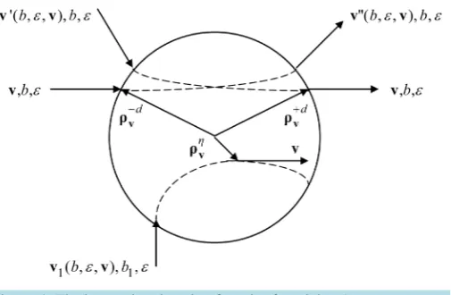
In Equation (2.4), the vectors ρ−_vd and ρ+_vd have the cylindrical coordinates b, , ε −d and b, , ε +d

respectivelyin the reference frame with the z axis parallel to the v vector, b is the impact parameter, and

ε

is the azimuthal angle. The 2

(

, 1, ,1 ,

)

d

F t x ξ ρ v+v function in the second term on the right hand side of Equa-tion (2.4) corresponds to a pair of particles 1 and 2, which leave the interacEqua-tion domain C₀

(

ρ ρ= +dv

)

at

ve-locities ξ₁ and ξ₂, Figure 1. The 2

(

, 1, ,1 ,

)

d

F t x ξ ρ v−v function in the second term on the left hand side of Equation (2.4) corresponds to a pair of particles 1 and 2, which enter the interaction domain C₀

(

ρ ρ= −vd

)

at

velocities ξ₁ and ξ₂.

Express the 2

(

, 1, ,1 ,

)

d

F t x ξ ρ v+v function in terms of the two-particle distribution function at the entrance to the domain C₀. To do this, it is expedient to pass from function F₂ to function F₂ written in x, ρ, G, v

variables. In accordance with Equation (2.2b), F t x G2

(

, , , ,ρ v

)

experiences changes of about O

( )

ν due to triple collisions of particles, as particles 1 and 2 travel in the domain C₀ along the 12-dimensional phase tra-jectory:

(

)

( )

2 , 1, 1, , 2 , 1 , , , 2 0, 1 0 , , , 1

2 2

d d

d d d

F t F t F t τ τ O ν

+ + + + − ′     ′ =  = − =  − = − − _{ } + _     v v

v v v

ρ ρ

x ξ ρ v x x G ρ v x x G G ρ v

   (2.5)

here, τ₀ is the time within which the particles traverse the interaction domain C₀, The cylindrical coordinates of the −d

′

v

ρ vector are b, , ε −d in the reference frame with the z axis parallel to v′= −ξ ξ₁′ ′₂. If particles 1 and 2 enter the C₀ at velocities ξ ξ ξ₁′

(

₁, ₂, ,bε

)

and ξ ξ ξ′₂

(

₁, ₂, ,bε

)

, v′= −ξ ξ₁′ ′₂, then they have velocities

1

ξ and ξ₂ respectively at the exit of the C₀, Figure 1. Further transformation of relations (2.5) gives:

( )

2 0 1 0 2 1

2 1 1

, , , , , , , , 1

2 2

, , , , 1

2 2 2

d d

d d

d d

d

F t F t O

F t O

τ τ + − + − ν

′ ′ + − − ′ ′     ′ ′ − = − − = = −  +     _{  }        _′ ′ _′ = _ − −  = + _ +     v v v v v v v ρ ρ

x x G Gρ v x x G ρ v

ρ ρ v

x ξ G ρ v

 

 _

_{( )}

ν _,

(2.6)

The _{2 0}, _{1 0} , , ,

2

d d

F t τ τ

+ − ′   ′ − = − −     v v ρ

x x G Gρ v

 function corresponds to a pair of particles 1 and 2, which

en-ter the inen-teraction domain C₀

(

ρ ρ= −vd′

)

. Function 2 0, 1 0 , , , 2

d d

F t τ τ

+ − ′   ′ − = − −     v v ρ

x x G Gρ v

[image:5.595.189.442.83.248.2]

Figure 1. The interaction domain of a pair of particles C0.

riant along the trajectory of the center of mass of a pair of particles to within O

( )

ν at the times, proportional to

d c. Weak dependence of the F t₂

(

, ,x G,ρ vv−′d, ′

)

function on l0-scale at the boundary of interaction domain 0

C is specified by weak dependence of the F₂p

(

t, ,x G,ρ v−v′d, ′

)

function on l0-scale, see Equations (3.10) and (3.11). Boundary condition (3.6) connects functions _F₂p _and

2 F .

Apply Equation (2.2b) to penetrate the domain C₀. Let vector ρη_v specifies any respective location of par-ticles in pair within the C₀ domain, Figure 1. The ρη_v vector has the cylindrical coordinates b, , ε η,

d η d

− ≤ ≤ + in the frame of reference with the z axis parallel to the v vector. Then,

(

)

(

₁

)

( )

2 , , , , 2 0, 0, , , 1 1

η d

F t x G ρ vv =F t −τ′ x G− τ′ G ρ v−v _ +O ν _ (2.7)

The pair of particles with the parameters b₁ and

ε

enters the domain C₀ at time t−τ ′₀

(

τ0′ <τ0

)

at ve-locity v₁

(

b, ,ε v

)

and reaches the location ρη_v by the time t, Figure 1.

Let us apply the operator

t

∂ ∂

 

∇ =_ + _

∂ ∂

 G x upon Equation (2.7). Function 2

(

0, 0, , 1, 1

)

d

F t −τ′ x G− τ′ Gρ v−v corresponds to a pair of particles, which enter the interaction domain C₀

(

ρ ρ= −vd′

)

. In accordance with the

aforesaid, function

(

)

1

2 0, 0, , , 1

d

F t −τ′ x G− τ′ G ρ v−v remains invariant along the trajectory of the center of mass of a pair of particles to within O

( )

ν at the times, proportional to d c. After action of the operator ∇, the left side of Equation (2.7) assumes the form:

(

)

( )

2 ˆ

ˆ _{, , , , 0}

ˆ ˆ

η

F t O

t ν

∂ ∂

 ₊  _{+ =}

_{∂ ∂} 

 G  x G ρ vv

x  (2.8)

Equation (2.8) is specified in terms of dimensionless time and coordinates on the initial scale. Recast Equa-tion (2.8) in terms of distribuEqua-tion funcEqua-tion F t x₂

(

, ₁,ξ ρ v₁, ,

)

, written in x₁, ξ₁, ρ, v variables, then

(

)

(

)

( )

1 2 1 1 2 1 1

1 1

ˆ ˆ ˆ

ˆ _{, , , , , , , , 0}

ˆ ˆ 2 ˆ

η η

F t F t O

t ν

 ∂ ∂  ∂

+ − + =

_{∂ ∂}  _∂

  v v

v

ξ x ξ ρ v x ξ ρ v

x x

 

  (2.9)

Upon substituting the third term on the left hand side of Equation (2.4) into the force term of the first equation of hierarchy (2.1), this equation assumes the form:

(

) (

)

(

) (

)

(

)

(

)

(

)(

)

0 0

1 1 1 1 2 1 1 2 1 1

1

1,3

1 2 1 1 3 3 3

1 1

, , 1 , , , , , , , , d d d

1 , , , , d d 1 2 d d d d ,

ˆ

d d

C C

F t N v F t F t b b

t

N F t N N F

t m

ε

+ −

∂ ₊ ∂  _{− −  − }

_{∂ ∂}  _{ }

 

 ∂ ∂    ∂

= − _ + _ + − − _{ }

∂ ∂ _{ }∂

 

∫

∫

∫ ∫

v v

ξ x ξ x ξ ρ v x ξ ρ v v

x

Ф

ξ x ξ ρ v ρ v x ξ v ρ

x ξ

 

 

 (2.10)

trajectory on the initial scale. Then, the F t x₁

(

, ₁,ξ₁

)

function varies in the order of own magnitude along this trajectory exclusively at the times, proportional to λ c, i.e., the first term on the left hand side of Equation (2.10) is of order

(

1Vc3

)

c λ. So is the second term on the left hand side of Equation (2.10).

To assess the order of magnitude of the first term on the right hand side of Equation (2.10) we use the Equa-tion (2.9). Generally, there are no reasons to believe that the F t x₂

(

, ₁,ξ ρ v₁, ,

)

function varies slightly with x₁

on the scale of particle size d, therefore, let us save for the first term on the right side of Equation (2.10) the order of

(

1Vc3

)

c λ. The order of the second term on the right hand side of Equation (2.10), allowing for triple collisions, is

(

1Vc3

)

cd λ2 .

Expand the dimensionless one-particle distribution function in a perturbation theory series in terms of the virial parameter ν:

(

)

( )

₍

₎

1 1 1 1 1 1

0

ˆ _{, ,} k ˆ k _{, ,}

k

F t ν F t

∞

=

=

∑

x ξ x ξ (2.11) Following Equation (2.11), expand functions Fˆ₂ and Fˆ₃ in a perturbation theory series. Substitute received series into the dimensionless Equation (2.10). Take into account the aforesaid estimates of the terms. Equating the multipliers at equal degrees of ν, let us specify the equation for Fˆ₁( )0

(

t x, ₁,ξ₁

)

. Omitting the superscript of distribution functions and going back to the dimensional quantities, one obtain:

(

) (

)

(

) (

)

1 1 1 1 2 1 1 1 2 2 1 1 1 2 2 1

1

, , 1 , , , d, , , , d, d d d

F t N v F t F t b b

t ε

+ −

∂ ∂  _{ }

+ = − − − − + ∆

_{∂ ∂}  _{ }

 ξ x  x ξ

∫

x ξ x ρ ξv x ξ x ρ ξv ξ (2.12)

(

)

(

)

0

1 2 1 1 1 2 2

1

1 , , , , d d

2 C

N ∂ F t

∆ = − −

∂

∫

v x ξ x ρ ξ ρ ξ

x

The transition (Equations (2.5) and (2.6)) from the F₂ function at the outlet of the C₀ interaction domain to that at the inlet of this domain in the first term on the right hand side of Equation (2.12) enables one to recast Equation (2.12) differently:

(

) (

)

(

) (

)

1 1 1 1 2 1 1 1 2 2 1 1 1 2 2 1

1

, , 1 , , , d, , , , d, d d d

F t N v F t F t b b

t ε

− −

′

∂ ₊ ∂  _{= −  ′ ′ ′− ′ − −  + ∆}

_{∂ ∂}  _{ }

 ξ x  x ξ

∫

x ξ x ρ ξv x ξ x ρ ξv ξ (2.13)

1 1

2 2

d d

+ −

′

 

′ = −_ − _

 

v v

ρ ρ

x x

In accordance with Equation (2.2а), F t x₁

(

, ₁,ξ₁

)

varies slightly along the ξ₁-particle trajectory at the times, proportional to d c. However, there are no reasons to believe that the F t x₁

(

, ₁,ξ₁

)

function varies slightly on the initial l₀-scale in space and with time separately. Assume that

(

)

(

)

(

)

(

)

1 1 1 3 1 1 1

2 1 1 1 2 3 2 1 1 1 2

1

, , , , d ;

1

, , , , , , , , d .

W

W

F t F t l

F t F t

l

= +

− = + −

∫

∫

x ξ x a ξ a

x ξ x ρ ξ x aξ x + a ρ ξ a

(2.14)

The spatial integration in Equation (2.14) is performed within the W region having the characteristic linear size l, d l λ. Averaging (2.14) removes the term ∆₁ on the right side of Equations (2.12) and (2.13) from the main order of magnitude. The averaged F t x₁

(

, ₁,ξ₁

)

and F t₂

(

,x₁,ξ x ρ ξ₁, ₁− , ₂

)

functions weakly change on the scale of particle size d. Because F t x₁

(

, ₁,ξ₁

)

and hence, F t x₁

(

, ₁,ξ₁

)

change only slightly with time along the particle trajectory on the initial l₀-scale, F t x₁

(

, ₁,ξ₁

)

varies slightly with time also on the initial scale. Analogously, the _{F t2}

(

, ₁, ₁, ₁₋ −d, ₂

)

v

x ξ x ρ ξ function varies slightly in space on the initial l₀-scale. The particles described by the _{F t2}

(

, ₁, ₁, ₁₋ −d, ₂

)

v

x ξ x ρ ξ function don’t enter the domain of their interaction C₀

(

₌ −d

)

v

ρ ρ . Thus, in accordance with Equation (2.2b), the _{F t2}

(

, ₁, ₁, ₁₋ −d, ₂

)

v

x ξ x ρ ξ function varies slightly with time also on the initial scale.

(

)

1 , 1, 1

F t x ξ distribution function marks the place in space in the vicinity of which a set of particles is concen-trated within an unit volume. Multiply the F t x₁

(

, ₁,ξ₁

)

function by the number of ways in which a pair of par-ticles can be selected from an ensemble of N particles:

(

)

(

)

1 , 1, 1 1 , 1, 1

f t x ξ =NF t x ξ (2.15) The one-particle distribution function f t x₁

(

, ₁,ξ₁

)

has the meaning of the probable number of particles si-tuated at time t in an unit volume element near point x₁ and having velocities in an unit interval near the ξ₁ point. Multiply Equations (2.12) and (2.13) by N, and average these equations over x₁ within region W :

(

)

(

) (

)

1 1 1 1 1 1

1

, , 1 , ,

f t N N J t t

∂ ∂ 

+ = −

_{∂ ∂} 

 ξ x  x ξ x ξ (2.16)

(

, 1, 1

)

(

, 1, 1, 2

)

d 2 J t x ξ =

∫

J t x ξ ξ ξ

In Equation (2.16) collision integral assumes the form:

(

, 1, ,1 2

)

2

(

, 1, ,1 1 , 2

) (

2 , 1, ,1 1 , 2

)

d d

d d

J t x ξ ξ =

∫

v F t_ x ξ x ρ ξ− +v −F t x ξ x ρ ξ− −v _b b ε (2.17a)

(

, 1, ,1 2

)

2

(

, 1, ,1 1 , 2

) (

2 , 1, ,1 1 , 2

)

d d

d d

J t x ξ ξ =

∫

v F t_ x ξ x ρ ξ′ − +v′ ′ −F t x ξ x ρ ξ− v− _b b ε (2.17b)

Recast collision integral J t x

(

, ₁,ξ ξ₁, ₂

)

(2.17b) in terms of two-particle distribution functions F₂, written in 1

x , ρ, G, v variables:

(

, 1, ,

)

2

(

, 1, , ,

) (

2 , 1, , ,

)

d d

d d

J t x G v =

∫

v F t_ x G ρ v−_v′ ′ −F t x G ρ v_v− _b b ε (2.18)

(

, 1, ,

)

(

, 1, ,1 2

)

J t x G v =J t x ξ ξ

The velocity G of the center of mass of pair particles and the modulus v of the relative velocity of par-ticles, v= v , are invariants of a binary particle collision. The enumeration of all the admissible target parame-ter values b and

ε

and the directions of relative motion velocity v at a fixed G and v values then gives all the possible velocity directions v′. It follows that a collision-caused decrease in the number of pairs of par-ticles from an unit phase volume interval near the x₁, , G v point characterized by all the admissible b and

ε

parameter values and relative motion v orientations is strictly balanced by a collision induced increase in the number of pairs of particles in this interval with these parameters,

(

)

2

1

, , , d 0

J t Ω =

∫

 x G v (2.19) here _d2_{Ω =sin d d}θ θ ϕ_{, and} θ _and ϕ _{are the spherical coordinates of the}

v vector.

Suppose that ϕ₂( )n

(

G,v

)

, n=0,1,, is an arbitrary weight function of velocities G and v. The pair properties of the ϕ₂( )n

(

G,v

)

, n=0,1,, are invariants of a particle binary collision. Let us multiply the

(

, 1, ,

)

J t x G v collision integral determined by Equation (2.18) by ϕ₂( )n

(

G,v

)

, n=0,1,, and integrate the result with respect to velocities. By virtue of Equation (2.19), we then have,

( )

₍

_{) (}

₎

2 , , 1, , d d 0 n

v J t

ϕ =

∫

G  x G v G v (2.20) This means that particle collisions cannot influence the formation of hydrodynamic values constructed on the properties of the ϕ₂( )n

(

G,v

)

, n=0,1,, pair. In other words, particle collisions cannot tune the distributions of all these hydrodynamic values to distributions of some other hydrodynamic values. That is, the set of hydrody-namic values constructed on the property of ϕ₂( )n

(

G,v

)

, n=0,1,,

( )

₍

₎

₍

₎

( )

₍

₎

(

)

1 n , 1 1 2 , 2 , 1, , , d d d d

n n d

i i

M  t x =N N− τ ϕ

∫

G v vF t x G ρ v−v b b ε G v (2.21)

is a set of the principal hydrodynamic values. The N N

(

−1

)

τ proportionality coefficient allows discovering the correspondence between the ( )

(

)

1 n , 1 n i i

reveals the existence of an infinite number of principal hydrodynamic values.

The equation for the f t x₁

(

, ₁,ξ₁

)

one-particle distribution function (2.16) is written in a six-dimensional phase space of one particle (µ space). The dimension of the µ space allows only the properties of a particle

( )

_{( )}

1 1

n

ϕ ξ , n=0,1,, to be accommodated in it; binary particle collision invariants, that is, ϕ₂( )n

(

G,v

)

, 0,1,

n= , do not fit into the µ space. Let us sequentially accommodate the properties of a particle ϕ₁( )n

( )

ξ₁ , 0,1,

n= , in the µ space. We then have:

( )

₍

₎

₍

₎

( )

₍

₎

1 1 1 1 1 1 1 1 1 1

1

, , d 1 , , d

n n

f t N N J t t

ϕ _∂ + ∂ _ = − ϕ

∂ ∂

 

∫

ξ x ξ ξ

∫

x ξ ξ

x (2.22)

It follows [3] that the integrals in the right hand side of (2.22) that contain the lower particle properties 1, ξ₁ and 2

1

ξ as weight functions are strictly reduced to the integrals with the 1, G,

(

G2+v2 4

)

weight functions belonging to ϕ₂( )n

(

G,v

)

n=0,1,, invariants. It follows that, according to Equation (2.20), these integrals are strictly zero. The integrals of all the other higher properties of a particle ϕ₁( )n

( )

ξ₁ different from 1, ξ₁ and 2

1 ξ are not zero [3].

It follows that, when we pass to the hydrodynamic stage from the phase space of one particle, such hydrody-namics equations cannot be constructed using more than three lower principal hydrodynamic values corres-ponding to the 2

1 1

1, , ξ ξ particle properties. The transition to the hydrodynamic stage from the phase space of one particle excludes higher principal hydrodynamic values (2.21) from participation in the construction of hy-drodynamics equations. However, there is no rigorous passage to hyhy-drodynamics from the µ space. This pas-sage is closed because Equation (2.16) is not closed.

The use of the Boltzmann hypothesis (“Stosszahlansatz”) opens up the possibility of approximate passage to hydrodynamics. Following Boltzmann, let us factorize two-particle distribution functions in the J t x

(

, ₁,ξ ξ₁, ₂

)

collision integral (2.17b):

(

)

(

) (

)

(

)

(

) (

)

2 1 1 1 2 1 1 1 1 1 2

2 1 1 1 2 1 1 1 1 1 2

, , , , , , , , ;

, , , , , , , , .

d

d

F t F t F t

F t F t F t

−

− ′

− =

′ − ′ = ′ ′

v

v

x ξ x ρ ξ x ξ x ξ

x ξ x ρ ξ x ξ x ξ

(2.23) Boltzmann hypothesis (2.23) closes Equation (2.16). The obtained classic kinetic equation for the f t x₁

(

, ₁,ξ₁

)

one-particle distribution function is called the Boltzmann equation [4]:

(

)

(

) (

)

(

) (

)

1 1 1 1 1 1 1 1 1 2 1 1 1 1 1 2 2

1

, , , , , , , , , , d d d

f t v f t f t f t f t b b

t ε

∂ ₊ ∂  _{=  ′ ′ − }

_{∂ ∂}   

 ξ x  x ξ

∫

x ξ x ξ x ξ x ξ ξ (2.24)

So, the physical meaning of the error introduced by the Boltzmann hypothesis (2.23) into hydrodynamics is as follows. It follows that just Boltzmann hypothesis allows us to construct hydrodynamics on only three lower principal hydrodynamic values. It follows that the use of the Boltzmann hypothesis excludes higher principal hydrodynamic values (2.21) from the participation in the formation of classic hydrodynamics equations. To in-clude the higher principal hydrodynamic values, we must find passage to hydrodynamics from the phase space capable of accommodating the whole set of binary particle collision ϕ( )₂n

(

G,v

)

, n=0,1,, invariants.

3. Equations for Pair Distribution Functions

The second equation of the BBGKY hierarchy (2.1), like the first one, is not closed. The integral term of the second hierarchy equation contains a three-particle distribution function responsible for interaction of particles 1 and 2 with some third particle 3. The absence of closeness of the second hierarchy equation prevents us from the direct transition to the hydrodynamic stage from the phase space of two particles.

Let us recast the second equation of the BBGKY hierarchy (2.1) in the trajectory form. Let particles 1 and 2 are located beyond the interaction domain С₀, then:

(

)

(

(

)

(

)

)

(

)

(

(

)

(

)

)

(

)

(

)

0

2 1 1 2 2 2 0 1 1 0 1 2 2 0 2

13

3 1 1 1 2 2 2 3 3 3 3

1

23

3 1 1 1 2 2

2

, , , , , , , ,

2 , , , , , , d d d

2 , , ,

t

t

F t F t t t t t

N F s t s t s s

m

N F s t s t

m

= − − − −

∂

− − − − − −

∂ ∂

− − − − −

∂

∫ ∫

x ξ x ξ x ξ ξ x ξ ξ

Φ

x ξ ξ x ξ ξ x ξ x ξ

ξ Φ

x ξ ξ x ξ

ξ

(

(

)

)

0

2 3 3 3 3 , , , d d d , t

t

s s

−

∫ ∫

ξ x ξ x ξ

In accordance with Equation (3.1), under absence of collisions with particle 3, particles 1 and 2, which at the time t₀ was located with a probability F₂ within an unit element of the phase space near the point

(

)

(

)

1− 1 t−t0 , , 1 2− 2 t−t0 , 2

x ξ ξ x ξ ξ , will be at time t within an unit element of the phase space near the point x₁, , , ξ x ξ_{1 2 2}. The second and the third terms on the right-hand side of Equation (3.1) are responsible for the interaction of particles 1 and 2 with particle 3 respectively. The second term on the right hand side of Equa-tion (3.1) has the meaning of probability that particle 1 experiences a collision with particle 3 during the time interval t−t₀

(

t−t0l c

)

. The third term on the right hand side of Equation (3.1) has the meaning of proba-bility that particle 2 experiences a collision with particle 3 during the time interval t−t₀

(

t−t0l c

)

. Based on the generally accepted assumption that a particle may be present at all phase space locations with equal probabilities, evaluate the contribution of the second and the third terms on the right side of Equation (3.1):

(

)

(

(

)

(

)

)

2 , 1, 1, 2, 2 2 0, 1 1 0 , 1, 2 2 0 , 2 1 l

F t F t t t t t O

λ

  

= − − − − _{ +  }

 

 

x ξ x ξ x ξ ξ x ξ ξ (3.2)

In accordance with Equation (3.2), the distribution function F₂ varies slightly along the trajectory of the two particles in 2µ-space on the scale of particle size

(

ld

)

. As the time interval t−t₀ grows, the error

( )

O l λ monotonically increases. On the scale of free path

(

lλ

)

, the error reaches the order of magnitude of the F₂ function itself. The arbitrariness in the location of particle 3 with respect to particles 1 and 2 in the second and the third terms on the right-hand side of Equation (3.1) is the cause of monotonic increase of the er-ror (3.2). When evaluating the order of magnitude of the terms in Equation (3.1), the assumption that a particle may be present at all phase space locations with equal probabilities was used for any position in space of par-ticles 1 and 2. However, there exist such mutual arrangements of parpar-ticles 1 and 2, for which the assumption on equality of probabilities gives a wrong estimation of the order of the second and the third terms on the right side of Equation (3.1).

Let us evaluate the typical number of particles N₁, which experience a binary collision within an unit space volume at any time moment t:

[ ]

0 2

1 2d d d1 2 C

N N  F 

 



∫ ∫

ξ ξ ρ 

In accordance with this estimation, the order of magnitude of N₁ is

[ ]

N₁ ∼1dλ2. Two particles take part in a collision, so the typical number of collisions N₁ within an unit space volume at any time t is N₁=N₁ 2. If the duration of the collision is τ₀

(

d c

)

, then the typical number of particles, which experience a binary col-lision within an unit space volume during the time of free path

(

λ c

)

equals N₂. The order of magnitude of

2

N is

[ ] [ ]

N₂ ∼ N₁ λ d, i.e.,

[ ]

N₂ ∼1d2λ. Therefore, the typical number of collisions N₂ within an unit space volume during the time of free path is N₂=N₂ 2. Let us multiply the second term on the right hand side of Equation (3.1) by N and integrate it with respect to x₂, ξ₂ and ξ₁. The N₂ value should be used to as-sess the order of magnitude of the received expression on the time scale, proportional to λ c.

In accordance with ideas of the kinetic theory of gases [14], the characteristic space volume per particle of gas medium

(

V N

)

is identified with a characteristic volume, which the particle covers during the time of free path

(

d2λ

)

. Then, during the time of free path

(

λ c

)

, N₃ particles in average experience a collision within the volume, proportional to d2λ,

(

[ ] [ ]

N₃  N₂ d2λ

)

. That is, during the time between collisions

(

λ c

)

, only one particle in average

(

[ ]

N₃ 1

)

experiences a collision within the space volume per one medium particle

[

] [

]

(

2

)

2 1

V N  N d λ . Then, during the time between collisions

(

λ c

)

, N₄ particles in average experience a collision within the volume V (

[ ]

N₄ 

[ ]

N₃ N, i.e., N₄ ~N). That is, during the time, proportional to λ c, each of medium particles in average experiences one collision. The error of the estimation δN₄ does not ex-ceed the typical number of triple collisions in medium during the time, proportional to λ c

(

δN4 ∼Nd λ

)

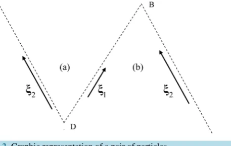
. Competition of the fluctuation error δN₄ is insignificant, δN ₄ N [15], δN ₄ δN₄ for N 1. The number of binary collisions within the volume V during the time, proportional to λ c, equals N 2.

In accordance with observations formed the ideas of the kinetic theory of gases on a free path, in a rarefied gas at each time moment, each particle after its last collision moves toward the next collision. This means that every particle 1 in a rarefied gas simultaneously flies away from some particle 2 with which it collided last at point D (Figure 2(a)) and approaches some particle 2 with which it is to collide next at point B (Figure 2(b)).

[image:10.595.209.438.85.230.2]

Figure 2. Graphic representation of a pair of particles.

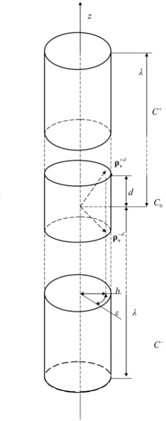
sion cylinder C+, ρ=

(

b, ,ε η

)

, 0≤ ≤b d, 0≤ ≤ε 2π, d≤ ≤η λ, Figure 3. The volume of the collision cy-linder C+

(

d2λ

)

equals to the average volume per particle of gas medium

(

V N

)

. Let at the time t₀,

(

t>t0

)

, particles 1 and 2, having collided, leave the domain of their interaction С0,

(

η=d

)

. At the time t0 the second term on the right hand side of Equation (3.1) describes a triple collision between particles 1, 2, and 3. During the collision time

(

t−t₀d c

)

, the order of the second term on the right hand side of Equation (3.1) will not exceed 1V c2 6

(

d λ

)

. In accordance with Equation (3.2), as time of motion of particles 1 and 2 in 2µ- space grows, contribution of the second term on the right hand side of Equation (3.1) increases monotonically. The probability that particle 1 will experience a collision with particle 3 becomes of the order of unity on the length of lλ. Monotonic increase (3.2) of the second term on the right hand side of Equation (3.1) contra-dicts the ideas of the kinetic theory of gases on a free path of particle. Indeed, particle 1 has already experienced collision with particle 2 at the time t₀ at the boundary of the collisions cylinder C+. Therefore, the rectilinear motion of particle 1 within the cylinder C+ must not be interrupted on the length of l

(

d≤ ≤l λ

)

. That is, the possibility of collision between particle 1 and particle 3 contradicts the above evaluated number of collisions

3

N within the cylinder C+. As a result, monotonic increase (3.2) of the second term on the right hand side of Equation (3.1) contradicts also the above evaluated number of collisions N₄ within the volume V . Indeed, in accordance with the estimation (3.2), the magnitude of N₄ reaches 2N that far exceeds the error δN₄ of the characteristic number of collisions (N₄ ~N,δN₄∼Nd λ). Thus, the assumption that a particle may be present at all phase space locations with equal probabilities sets too high estimation of the second term on the right hand side of Equation (3.1). Estimation of the second term on the right side of Equation (3.1) requires a more accurate evaluation of the order of magnitude of the F₃ function. The aforesaid estimations are fully applicable to the third term on the right hand side of Equation (3.1). Let the F₂p( )+ function describes particles 1 and 2 located within the collision cylinder C+. Then, based on the estimation of the number of collisions N₃ within the cy-linder C+ during the time, proportional to λ c, we have :

( )

₍

₎

( )

₍

₍

₎

₍

₎

₎

_{( )}

2 , 1, 1, 2, 2 2 0, 1 1 0 , 1, 2 2 0 , 2 1

p p

F + t x ξ x ξ =F + t x −ξ t−t ξ x ξ− t−t ξ _ +O ν _ (3.3) Equation (3.3) has a clear physical meaning. It asserts that a pair of flying-apart particles, that is, of particles that have already left the domain of their interaction C₀ and are located within the cylindrical volume C+, travels undergoing no collisions with third particle 3. Note that the ideas of the kinetic theory of gases on the free path of particle are valid for an arbitrary gas particle at every time moment. That is why, partial distribution functions Fs, 1,s= ,N, themselves rather than fluctuations of these functions must correspond to these ideas.

Let particles 1 and 2 are located so that at time t the vector ρ x x= ₁− ₂ does not extend beyond the colli-sion cylinder C−, ρ=

(

b, ,ε η

)

, 0≤ ≤b d, 0≤ ≤ε 2π, − ≤ ≤ −λ η d, Figure 3. The volume of collision cy-linder C−

(

∼d2λ

)

equals to the average volume per particle of gas medium

(

V N

)

. Let at the time t₀,

(

t<t0

)

, particles 1 and 2 reach the domain of their interaction С0,

(

η= −d

)

. At the time t0 the second term on the right hand side of Equation (3.1) describes a triple collision between particles 1, 2, and 3. During the col-lision time

(

t₀−td c

)

, the order of the second term on the right hand side of Equation (3.1) will not exceed

(

)

2 6

[image:11.595.234.404.85.515.2]

Figure 3. The interaction domain of a pair of particles C0, the collision cylinders C− and C+.

Monotonic increase (3.2) of the second term on the right hand side of Equation (3.1) contradicts the ideas of the kinetic theory of gases on a free path of particle. Indeed, particle 1 will experience collision with particle 2 at the time t₀ at the boundary of the collision cylinder C−. Therefore, the rectilinear motion of the particle 1 within the cylinder C− must not be interrupted on the length l

(

d ≤ ≤l λ

)

. As a result, the possibility of collision between particle 1 and particle 3 contradicts both the above estimated number of collisions N₃ within the cy-linder C− and the number of collisions N4 within the volume V. Thus, the assumption that a particle may be present at all phase space locations with equal probabilities sets too high estimation of the second term on the right hand side of Equation (3.1). Evaluation of the second term on the right side of Equation (3.1) requires a more accurate estimation of the order of magnitude of the F₃ function. The aforesaid estimations are fully ap-plicable to the third term on the right hand side of Equation (3.1). Let the F₂p( )− function describes particles 1 and 2 located within the collision cylinder C−. Then, based on the estimation of the number of collisions N₃

within the cylinder C− during the time, proportional to λ c, we have:

( )

₍

₎

( )

₍

₍

₎

₍

₎

₎

_{( )}

2 , 1, 1, 2, 2 2 0, 1 1 0 , 1, 2 2 0 , 2 1

p p

Equation (3.4) has a clear physical meaning. It asserts that a pair of drawing together particles, that is, of par-ticles that have not yet reached the domain of their interaction C₀ and are located within the cylindrical volume

C−, travels undergoing no collisions with third particle 3.

Let particles 1 and 2 are located so that at time t the vector ρ=x₁−x₂ does not extend beyond the domain of their interaction C₀, ρ=

(

b, ,

ε η

)

, 0≤ ≤b d, 0≤ ≤ε 2π, −d≤ ≤η d, Figure 3. Let distribution function

( ) 2 0 p

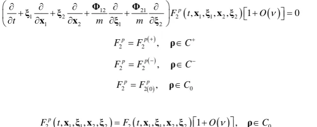
F describes particles 1 and 2 located within the interaction domain С₀. The evolution of the F_{2 0}p_{( )} function occurs at the times, proportional to d c. The second equation of the hierarchy (2.1) on the initial l₀-scale has the form (2.2b), in which Fˆ₂ can be replaced by F_{2 0}p_{( )}. Let F₂p equals the Fˆ₂p( )+ function within the collision cylinder C+, and the Fˆ₂p( )− function within the collision cylinder C−, and the function F_{2 0( )}p within the interac-tion domain C₀. Then:

(

)

( )

12 21

1 2 2 1 1 2 2

1 2 1 2

, , , , 1 0

p

F t O

t m m ν

∂ ₊ ∂ ₊ ∂ ₊ ∂ ₊ ∂  _{ + =}

_{∂ ∂ ∂ ∂ ∂}   

 

Φ Φ

ξ ξ x ξ x ξ

x x ξ ξ (3.5)

( )

2 2 ,

p p

F =F + ρ∈C+

( )

2 2 ,

p p

F =F − ρ∈C−

( )

2 2 0, 0

p p

F =F ρ∈C

here,

(

)

(

)

( )

2 , 1, ,1 2, 2 2 , 1, ,1 2, 2 1 , 0

p

F t x ξ x ξ =F t x ξ x ξ _ +O

ν

_ ρ∈C (3.6)

Generally, any medium particle forms a pair with every other particle. A medium therefore contains

(

1

)

N N− pairs of particles. All these pairs are described by the F t x₂

(

, ₁,ξ x ξ₁, ₂, ₂

)

function, which obeys the second equation of the BBGKY hierarchy (2.1). If a single particle 2, which either flies away from (Figure 2(a)) or approaches (Figure 2(b)) some particle 1, is selected as a partner of this particle, this pair is described by the

(

)

2 , 1, ,1 2, 2

p

F t x ξ x ξ function that obeys Equation (3.5). Note that Equation (3.5) is valid for an arbitrary gas par-ticle rather than some particular parpar-ticle 1 (Figure 2). Generally, a medium contains N 2 pairs of approaching particles, and N 2 pairs of diverging particles. For this reason, Equation (3.5) is capable of describing the gas as a whole. Heuristic derivation of Equation (3.5) was given in [3]. In [11], Equation (3.5) was derived in terms of conditional probabilities. In accordance with [11], the ₂p

F distribution function is limited by the condition that the third particle is not located within the collision cylinders C+ and C−, Figure 3. Earlier, the formalism of conditional probabilities was used in [16] in deriving the Boltzmann equation for a gas consisting of rigid spheres.

Expand the dimensionless two-particle distribution function in a perturbation theory series in terms of the virial parameter ν:

(

)

( )

₍

₎

2 1 1 2 2 2 1 1 2 2

0

ˆp _{, , , ,} k ˆp k _{, , , ,} k

F t ν F t

∞

=

=

∑

x ξ x ξ x ξ x ξ (3.7)

Let us substitute Equation (3.7) into the dimensionless Equation (3.5). Equating the multipliers at equal de-grees of

ν

, let us specify the equation for Fˆ₂p( )0

(

t x, ₁, ,ξ x ξ_{1 2}, ₂

)

. Let us omit the superscript of

( )0

₍

₎

2 1 1 2 2

ˆp _{, , , ,}

F t x ξ x ξ and go back to the dimensional quantities. Recasting the two-particle distribution function in variables x, ρ, G, v, one obtains:

(

)

12 2 2

, , , , 0 p

F t

t m

∂ ₊ ∂ ₊ ∂ ₊ ∂  ₌

_{∂ ∂ ∂ ∂} 

 

Φ

G v x G v ρ

x ρ v  (3.8)

Integrating Equation (3.8) with respect to ρ over the cylindrical volumes C+ and C− yields

(

)

2π

(

)

(

)

div

2 2

0 0

, , , , , , , , , , , d d

d

p d p

p

F t v F t F t b b t

λ _ε

+ +

∂ ∂

 ₊  _{=  − }

_{∂ ∂}  _{ }

 G  x G v

∫ ∫

x G v ρv x G vρv

x   (3.9a)

(

)

2π

(

)

(

)

app

2 2

0 0

, , , , , , , , , , , d d

d

p p d

p

F t v F t F t b b

t

λ _ε

− −

∂ ∂

 ₊  _{=  − }

_{∂ ∂}  _{ }

 G  x G v

∫ ∫

x G v ρv x G v ρv

[image:12.595.153.480.211.342.2]