Phase relationships between two or more interacting processes from one-dimensional time series.
I. Basic theory
N. B. Janson,1A. G. Balanov,1 V. S. Anishchenko,2and P. V. E. McClintock1 1Department of Physics, Lancaster University, Lancaster, LA1 4YB, United Kingdom 2Department of Physics, Saratov State University, Astrahanskaya 83, 410026, Saratov, Russia 共Received 14 March 2001; revised manuscript received 27 July 2001; published 15 February 2002兲
A general approach is developed for the detection of phase relationships between two or more different oscillatory processes interacting within a single system, using one-dimensional time series only. It is based on the introduction of angles and radii of return times maps, and on studying the dynamics of the angles. An explicit unique relationship is derived between angles and the conventional phase difference introduced earlier for bivariate data. It is valid under conditions of weak forcing. This correspondence is confirmed numerically for a nonstationary process in a forced Van der Pol system. A model describing the angles’ behavior for a dynamical system under weak quasiperiodic forcing with an arbitrary number of independent frequencies is derived.
DOI: 10.1103/PhysRevE.65.036211 PACS number共s兲: 05.45.Xt, 05.45.Tp, 87.19.Hh
I. INTRODUCTION
To establish from experimental data whether or not two or more interacting processes are synchronized is an old and important problem. In the absence of noise, the existence of synchronization between two processes in interacting limit cycle oscillators was originally taken to imply that their basic frequencies of oscillation are related as integer numbers共i.e., are rationally connected兲 关1,2兴, and that their instantaneous phases are permanently locked. This definition suggests that the detection of whether or not synchronization exists can be established by computation of the ratio of basic frequencies in the Fourier spectrum of the signal from one of the sub-systems involved. Even in this simplest case, however, the finite observation time and the discreteness of the digitiza-tion steps used in practice will make it appear that all fre-quencies are rationally connected, thereby complicating the reliable estimation of their ratio. Furthermore, the noise that is invariably present in all real macroscopic systems means that only effective synchronization 关3兴 can normally take place, meaning that the phases can remain locked only dur-ing finite time intervals, and that the basic frequencies may no longer be rationally connected 关4兴. Serious difficulties may also arise due to the nonstationarity of experimental data.
In view of these problems, modern techniques for estab-lishing the presence or absence of synchronization are based on the assumption that the behavior of each subsystem can be considered separately, and that their individual time series can be compared by a variety of techniques共e.g., by compu-tation of the phase difference between them兲. This approach has been justified theoretically 关3– 6兴 and is widely used to detect synchronization, not only in periodic noisy, but also in chaotic关7–10兴oscillators, and even between stochastic关11– 15兴 processes. Its principal assumption is quite reasonable where the system is being forced externally, when one is able to measure both the forcing and response signals关16兴, or for mutually coupled oscillators of radiotechnical 关8,9,17兴 or biological关18兴origin, or for biological systems such as
iso-lated neurons关19兴, or in any situation when a living system is artificially split into separate subsystems for research pur-poses, usually by means of surgery or drugs共thereby disrupt-ing its natural functional state兲 关20–23兴. However, in practice there are not many opportunities to measure noninvasively separate signals coming from different interacting processes within a living system: the independent registration of sig-nals derived from respiration and from cardiac activity关24 – 28兴is one of the very rare examples.
It remains an open problem how best to learn from the one-dimensional signal coming from a system, within which several processes with distinguishable time scales interact, whether or not the processes in question are synchronous. In Ref.关29兴it was suggested that the interaction of processes in the autonomic regulation of the human cardiovascular sys-tem could be studied by the application of ideas from ethno-musicology to univariate time series共heart rate data兲. How-ever, this approach is tightly linked to the physiological nature of the particular data and cannot be applied in general. Another possibility that has recently been demonstrated关30兴 is to filter a univariate time series to create two ‘‘separate’’ signals that can then be analyzed for synchronization phe-nomena in the usual ways already developed for bivariate time series.
In the present paper we propose a more general approach towards detecting the presence or absence of synchronization between two or more interacting processes from univariate experimental data. A preliminary report 关31兴introducing the main idea has already been published. The aims of the present paper are, first, to give an explicit relation between the new variable introduced for univariate data and the con-ventional variables used in synchronization theory. Second, we extend the approach to encompass the case of several interacting processes.
oscillations and the method is tested. The results are summa-rized and discussed in Sec. IV, and conclusions are drawn in Sec. V.
II. ANALYTIC DESCRIPTION FOR THE IDEAL NOISE-FREE CASE
A. General idea and experimental observations
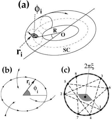
The central idea of the proposed approach is based on the simple fact that, if m periodic processes with different fre-quencies interact weakly enough within a single system, an m-dimensional torus exists in its phase space关2兴. The case of two interacting processes is illustrated by Fig. 1共a兲, showing a two-dimensional torus as the attracting set. To quantify motion on this torus, the rotation numberis introduced as the ratio between the basic frequencies of the interacting os-cillators. It specifies how many periods of one oscillator fall within a single period of the other oscillator.
If the processes are not synchronous, the rotation number is irrational. The phase trajectory then fills the whole torus surface and is never closed, and thus its Poincare´ map is a closed curve. If the processes are synchronous, the rotation number is rational. In this case, distinct stable and unstable cycles lie on the torus surface, and the phase trajectory tends towards the stable limit cycle. The Poincare´ map consists of one or several stable points belonging to the stable cycle and an equal number of saddle points belonging to the saddle cycle lying between the stable points on the closed curve
formed by the unstable manifolds of the saddles as shown in Fig. 1共b兲. To consider the dynamics of the Poincare´ map, place the origin somewhere inside the region bounded by the closed curve and introduce the phase angle i and phase radius ri 关Fig. 1共b兲兴. At each discrete time moment ti when
the trajectory returns to the Poincare´ secant surface, the phase vector rotates by some angle. It is obvious that for the synchronous regime there is a discrete number of possible values ofi, and for the asynchronous one the angleimay take any value between 关⫺;兴. The geometrical meaning of the rotation number is then the average angle by which the phase vector rotates at each step关Fig. 1共c兲兴,
具
i⫺i⫺1典⫽2, 共1兲where具¯典means an average over time.
If some general noise共with large enough tails in its dis-tribution兲perturbs the system, only effective synchronization can take place 关3兴. In terms of the Poincare´ section this means that, at every step, noise prevents the phase point from jumping exactly to the stable point, but makes it jump instead to the vicinity of the stable point. However, at a certain moment, a large enough fluctuation may throw the phase point outside the region bounded by the two stable manifolds of the nearest saddle points, and the phase point then moves along the unstable manifold to another stable point关Fig. 1共b兲兴. The latter stage of the dynamics is associ-ated with phase slip. Thus, instead of one or a few discrete points, one observes one or a few clouds of points smeared around the stable equilibrium/equilibria, and possibly also the trace of the unstable manifolds forming the torus. The latter situation is illustrated by Fig. 2共a兲where a stroboscopic section is shown for a Van der Pol system under harmonic forcing while affected by Gaussian white noise,
x˙⫽y ; y˙⫽⑀共1⫺x2兲y⫺
0x⫹C sin⍀t⫹
冑
D共t兲. 共2兲 Here, the nonlinearity parameter ⑀⫽0.1, eigenfrequency0⫽1, forcing amplitude C⫽0.1, forcing frequency ⍀
⫽1.025, (t) is a random value with a Gaussian distribu-tion, zero average and unity variance, and the noise variance D⫽0.1. For these parameter values, effective 1:1 synchroni-FIG. 1. 共a兲Surface of a two-dimensional torus. The point O is
some origin in whose vicinity the motion occurs. The saddle cycle SC共dashed line兲is that from which the torus was created as a result of a Hopf bifurcation. The phase trajectory moves along the torus surface and makes two kinds of rotation: around the point O with amplitude R, and around the cycle SC with amplitude r.共b兲 Poin-care´ map for a two-dimensional resonant torus inside the region of 1:3 synchronization. Arrows show the direction of stable and un-stable manifolds of saddle equilibria.iis the current angle, ri is
[image:2.612.329.548.57.166.2]the current amplitude. 共c兲 Illustration how the points jump on the Poincare´ section of a two-dimensional torus.
FIG. 2. 共a兲Stroboscopic section of a Van der Pol system forced periodically and influenced by noise in the region of 1:1 effective synchronization 共black points兲. The white point shows the stable cycle in the noise-free system. Parameter values are given in the text.共b兲 Map for angles of return times for the case illustrated by
共a兲. The thin black line shows the return function of Eq. 共11兲 for
[image:2.612.77.273.58.268.2]zation takes place. In Fig. 2共a兲black points show the strobo-scopic map of system with noise, and the white diamond in among the bulk of the black ones shows the position of the stable cycle in the noise-free system. Here, the anglei can take any possible values, but those corresponding to the vi-cinity of stable equilibrium are the most probable. Effective synchronization manifests itself in a sharp increase in the duration of the time intervals without phase slips.
According to the Takens theorem关32兴and its extension to noise-affected system 关33兴, the system’s attractor can be re-constructed from its one-dimensional time series. Obviously, the Poincare´ map can also be restored from the reconstructed phase trajectory, being topologically equivalent to that of the original system. In Refs. 关34,35兴 it is shown that the same map can be reconstructed from return times of the system.
Consider a map for the angles of a return times map,
i⫽f共i⫺1兲. 共3兲
The technique of plotting such a map has already been ap-plied to reveal determinism in the R-R intervals of anesthe-tized dogs 关36兴 and in the human heart rate during paced respiration 关37兴, and in jet atomization关38兴. The distinctive shape of the maps observed in all these works was attributed to interaction between the particular processes involved. Her-zel et al. 关36兴 and Suder et al. 关37兴 suggested approximate empirical models to describe the dynamics of such maps, but without linking them to the general theory of synchroniza-tion or developing an analytic descripsynchroniza-tion.
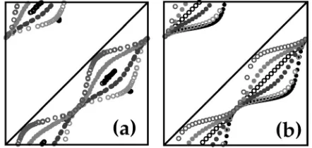
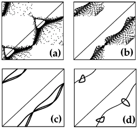
Some typical examples of such a map are shown in Fig. 3共a兲 for the noise-free Van der Pol system 共2兲 with⑀⫽0.1 and the small forcing amplitude C⫽0.01, for several values of forcing frequency ⍀varying from 0.25 to 0.9. The basic frequency of the oscillations is close to 0⫽1, and thus the rotation numbers are close to the corresponding values of ⍀. Note that, for⫽1/2, one observes a 1:2 synchronization that is reflected by the presence of only two points in the map of Fig. 3共a兲 共the most distant point from the diagonal in the lower-right part of the picture and the closest point to the diagonal in the upper-left part兲, and that the whole return function is not seen here since we removed all transients. All
the other regimes appear not to fall within the synchroniza-tion tongues. Here and in what follows, the axes of the maps for angles have the limits 关⫺;兴.
B. Derivation of the map for angles of return times map for two interacting processes
In this subsection we will clarify the physical meaning of the angles of return times map and will relate it to the con-ventional phase difference. We will also derive the map de-scribing the evolution of angles with time.
Consider a very simple case of a forced system, namely, a periodic self-sustained oscillator with eigenfrequency0and amplitude R that is forced harmonically at frequency⍀and amplitude r. As a result of the forcing, a two-dimensional torus is born关Fig. 1共a兲兴. If the nonlinearity in the oscillator is weak, its autonomous solution can be approximated by a sinusoidal function of time, and the oscillator is then called quasiharmonic. If the harmonic forcing is also weak, rⰆR, the solution of the resulting nonautonomous equations can be approximated by a superposition of: one sine term coming from the unforced system and describing rotation around some origin O, i.e., oscillations with frequencyand ampli-tude R 关as shown in Fig. 1共a兲兴; and a second sine term cor-responding to rotation around the saddle cycle 共SC兲 共the former limit cycle of the autonomous system from which the torus was born via a Hopf bifurcation兲, i.e., oscillations with the frequency of external forcing⍀and amplitude r. Thus
x共t兲⫽R sint⫹r sin共⍀t⫹0兲, rⰆR, 共4兲
where 0 is the initial phase shift. Note that frequency coincides with the eigenfrequency 0 of the autonomous system in the absence of synchronization. In the presence of synchronization, it is shifted in the direction defined by the forcing. If the oscillations are synchronized by the forcing, the rotation number of the whole system under consideration, here denoted as ⫽⍀/, is equal to n/m, where n, m are integers.
Define the return times of the system as the time intervals between successive crossings by the signal x(t) of a thresh-old x⫽0 in one direction. To find the time moments tk of
these crossings one should solve the transcendental equation x(t)⫽0, which in general has no analytic solution. Let us make use of the fact that the first term is much larger than the second one, and, therefore, that the times tkof zero crossing
by x(t) are close to the times tk*⫽k/ of zero crossing by (R sint). We expand the function x(t) as a Taylor series in the vicinity of tk*, considering only the linear term and
ne-glecting all the others:
x共t兲⫽R sink⫹r sin
冉
⍀ k⫹0
冊
⫹R冉
t⫺k
冊
cosk⫹r⍀
冉
t⫺k
冊
cos冉
⍀
k⫹0
冊
⫽0. [image:3.612.64.285.59.164.2]Noting that cosk⫽(⫺1)k, and in order to consider every second zero crossing so as to register intersections in only one direction, we set k⫽2i,
FIG. 3. 共a兲 Map for angles of return times for the Van der Pol system under periodic forcing with fixed small amplitude and dif-ferent values of rotation number.共b兲A series of return functions of map共11兲for different values of rotation numberclose to those in 共a兲. Moving down from the diagonal, the plots sequentially corre-spond to关according to relation共12兲兴:⫽0.1共and 0.9兲,⫽0.2共and 0.8兲, ⫽0.25 共and 0.75兲, ⫽0.3 共and 0.7兲, ⫽0.4 共and 0.6兲,
冉
t⫺2i
冊冋
R⫹r⍀cos冉
2i⍀
⫹0
冊册
⫽⫺r sin 2i⍀ .
The t we seek is the ith moment of crossing,
ti⫽⫺
r sin
冉
2i⍀ ⫹0
冊
R⫹r⍀cos
冉
2i⍀ ⫹0
冊
⫹2i. 共5兲
Divide the numerator and denominator of the first term of Eq. 共5兲 by r. Since RⰇr, and thus in the denominator the first term is much larger than the second one, we neglect the second term and thus obtain
ti⬇⫺
r
Rsin⌿i⫹ 2i
, 共6兲
where ⌿i⫽(2i⍀/⫹0). Denote ⍜⫽2⍀/⫽2. Then the expressions for the time moments ti, ti⫹1, ti⫹2, ti⫺1 may be written by analogy. The return times Ti are the
differences between the successive times ti:
Ti⫽ti⫹1⫺ti⫽⫺2
r
Rcos
冉
⌿i⫹ ⍜2
冊
sin ⍜2 ⫹ 2
.
Put the origin into the central point of the return times map (Ti,Ti⫹1) found as an average of all values Ti which is
equal to 2/. Introduce the angle between the current point and the horizontal axis as follows:
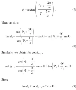
i⫽arctan
冉
Ti⫹1⫺2
Ti⫺
2
冊
. 共7兲
Then taniis
tani⫽
cos
冉
⌿i⫹3⍜ 2
冊
cos
冉
⌿i⫹⍜ 2冊
⫽cos⍜⫺tan
冉
⌿i⫹⍜ 2
冊
sin⍜.共8兲
Similarly, we obtain for coti⫺1,
coti⫺1⫽
cos
冉
⌿i⫺⍜ 2
冊
cos
冉
⌿i⫹⍜ 2
冊
⫽cos⍜⫹tan
冉
⌿i⫹⍜ 2
冊
sin⍜.Since
tani⫹coti⫺1⫽2 cos⍜, 共9兲 we obtain the following expression for the rotation number:
⫽ 1
2arccos
tani⫹coti⫺1
2 共10兲
and an explicit form of the map 共3兲for anglesi:
i⫽arctan共2 cos 2⫺coti⫺1兲. 共11兲 Equations共10兲and共11兲are the final formulas关39兴 connect-ing two successive angles of the return times map with the rotation number in the approximation of a quasiharmonic oscillator under weak harmonic forcing. Note that Eq. 共11兲 was quoted earlier as Eq. 共6兲 of Ref. 关31兴, without detailed justification.
C. Analysis of angles for two interacting processes First, note that, if the amplitude of forcing is much smaller than the amplitude of natural oscillations in the sys-tem, the map 共3兲does not depend on the amplitudes and is completely defined by the rotation number. The ambiguity in defining the value of arctan that is periodic with the period
, not 2, implies that the return function in Eq.共11兲is not continuous but makes a jump by at the point ⫽0, thus being not one-to-one. Moreover, the function arctan itself varies between ⫺/2 and /2. To draw the return function for angles in a proper way, reflecting its distinct physical meaning, we just leave the value ofiifi⫺1⭓0 and sub-tractfromi ifi⫺1⬍0. When referring to maps共11兲, or 共19兲 below, we will assume them to have been extended by this procedure.
Second, note that the map 共11兲 does not depend on the initial phase shift0 between the solution components.
Third, note that the return function of Eq.共11兲is periodic with respect to the variable with period 1, because the cosine function takes equal values for the arguments 2, or 2⫾2, or 2l⫾2 共where l is an integer兲 if 0⭐ ⭐1. Denote *⫽(1/2)arccos(cos 2), so that * or (1
⫺*) is the fractional part of the true rotation number lying within the interval关0;1兴. Then the true rotation numbercan be expressed via *as
⫽*⫹l, or ⫽共1⫺*兲⫹l. 共12兲
Thus, from the map for angles only * can be defined. To select one of the two formulas in Eq. 共12兲 and find l, the Fourier spectrum of the original signal x(t) can be helpful, since for this purpose only a rough estimate of the basic frequencies is required. To simplify further consideration, we will taketo mean the value of*which in all numerical or real data examples given in this paper coincides with true rotation number.
Fourth, it follows from Eq. 共11兲 that 共i兲 if ⫽1/4, the return function is the straight linei⫽i⫺1⫺/2共ii兲for any value of the return function passes through the points 共0;
⫺/2兲and 共;/2兲 and touches the linei⫽i⫺1⫺/2 at these points.
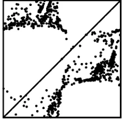
[image:4.612.47.297.425.721.2]Our numerical simulation has demonstrated that closely similar angles maps appear in the case when two periodic oscillators are coupled mutually and weakly; they are not shown here because they are equivalent to those for the forced Van der Pol system共2兲for the same rotation numbers 关Fig. 3共a兲兴. Another useful observation is that even in the case when a weakly chaotic oscillator is forced periodically, the map for angles may sometimes look very similar to that for noise-influenced forced or interacting periodic oscillators. In Fig. 4 a map for angles of return times is given for the Ro¨ssler oscillator 关40兴 in a chaotic regime forced periodi-cally. The form of the equations is taken to be as in关41兴with the following parameters values: eigenfrequency ⫽1; ␣
⫽0.2; ⫽0.2; ⫽10; and the forcing frequency 1⫽0.3 with amplitude C⫽0.5.
To reveal the physical meaning of the angles, return to Eq. 共8兲. Here, ⌿i is the phase of external forcing taken at the time moments 2i/ when the phase of basic oscillations with frequency changes by 2. Note that in general ⌿i
defines the phase of external forcing up to some constant. If ⌿i is wrapped into the interval 关⫺;兴 关which does not
change the value of tan(⌿i⫹/2)兴, it is by definition the so-called relative phase introduced in Ref.关25兴. Consider the phase difference between two signals, ⌿˜ (t)⫽⌽1(t)
⫺⌽2(t), and the values of⌿˜ at time moments ti when the
phase of one signal, e.g.,⌽2, changes by 2,
⌿˜共t
i兲⫽⌿˜i⫽⌽1共ti兲⫺2i. 共13兲
Wrapping of ⌿˜i into the interval 关⫺;兴 implies ⌿˜i
⫽⌽1(ti). That is, by construction, ⌿˜i coincides with ⌿i.
Thus, Eq.共8兲provides an explicit relation between the angles of return times map and the conventional phase difference up to some constant. This relation will be demonstrated by nu-merical simulation of a nonstationary process in Van der Pol system in Sec. III B.
A classical sine circle map关42兴is usually used to describe the evolution of phase difference⌿˜i:
⌿˜
i⫹1⫽⌿˜i⫹␦⫹K sin⌿˜i 共mod 2兲, 共14兲
where K is the effective amplitude of external forcing and␦ is the frequency detuning between the eigenfrequency of the
system and the external forcing. A typical return function of the map共14兲is shown in Fig. 5. Let us make a comparison of map共11兲with map共14兲.
The formal difference between Eq.共11兲and the sine circle map is the presence of two points at which the distance be-tween the return function and the diagonal is minimal, in-stead of only one such point. An important distinction is that the map 共11兲, unlike map 共14兲, does not depend on the am-plitude of forcing and is thus always one-to-one, so no chaos can be described by it. Another important feature is that the return function of Eq.共14兲can cross the diagonal, as param-eters K and ␦ are varied, while in the map 共11兲 it can only touch the diagonal at two points where ⫽0 or ⫽1, but never crosses it.
It is obvious that, when共i兲the approximation of a quasi-harmonic oscillator is not valid, and/or 共ii兲 the oscillator is not being forced harmonically, and/or 共iii兲 the amplitude of forcing cannot be considered small, the real map will differ from that predicted theoretically. However, even where one or more of共i兲–共iii兲apply, but the torus still exists, the quali-tative picture remains the same, i.e., for the synchronous re-gime we will obtain a finite number of points, whereas for the asynchronous one the map will look like a continuous curve.
We have, therefore, arrived at a diagnostic criterion for the existence of synchronization, or the lack of it, between two noise-free interacting processes manifested within a one-dimensional signal.
D. Derivation of map for angles for several interacting processes
We now consider the case when a quasiharmonic oscilla-tor is being forced, not just by one, but by n harmonic signals with n independent frequencies ⍀i, i⫽1, . . . ,n. We
sup-pose the amplitude Ai of each of these signals to be much smaller than R. Then, as before, the solution of the resulting nonautonomous system can be approximated by
x共t兲⫽R sint⫹
兺
j⫽1
n
Ajsin共⍀jt⫹j
0兲
, AjⰆR. 共15兲
Here j0 are the initial phase shifts of the solution compo-nents. Denote 2⍀j/⫽⍜j. As before, expand Eq. 共15兲 into Taylor series in the vicinity of ti*⫽2i/ and neglect all terms beyond the linear ones,
[image:5.612.112.236.59.180.2]FIG. 4. Map for angles of return times for the periodically forced Ro¨ssler system in a chaotic regime. The parameter values are given in the text.
x共t兲⫽
兺
j⫽1
n
Ajsin共i⍜j⫹j
0兲⫹
冉
t⫺2i
冊
⫻
冉
R⫹兺
j⫽1
n
Aj⍀jcos共i⍜j⫹j
0兲
冊
⫽ 0,to obtain an approximate expression for the moments ti of
the signal’s intersection with the zero axis,
ti⫽⫺
兺
j⫽1
n
Ajsin共i⍜j⫹j
0兲
R⫹
兺
j⫽1
n
Aj⍀jcos共i⍜j⫹j
0兲
⫹2i
⬇⫺R1
兺
j⫽1
n
Ajsin共i⍜j⫹j
0兲⫹2i
.
The return times are defined as
Ti⫽ti⫹1⫺ti⫽
2
⫺
1 R
冋
j兺
⫽1n
Ajsin共i⍜j⫹j
0⫹⍜
j兲
⫺
兺
j⫽1
n
Ajsin共i⍜j⫹j
0兲
册
⫽2⫺R2
兺
j⫽1
n
Ajcos
冉
i⍜j⫹j0⫹⍜j 2
冊
sin⍜j
2 .
Then taniis equal to
tani⫽ Ti⫹1⫺
2
Ti⫹2
⫽j
兺
⫽1n
jcos
冉
i⍜j⫹j0⫹3⍜j
2
冊
兺
j⫽1
n
jcos
冉
i⍜j⫹j0⫹⍜j
2
冊
,wherej⫽(Aj/A1)关sin(⍜j/2)/sin(⍜1/2)兴, 1⫽1. Transform the latter expression to rewrite it in a more convenient form,
tani⫽
冋
兺
j⫽1n
jcos
冉
i⍜j⫹j0⫹⍜j
2
冊
cos⍜j⫺j兺
⫽1n
sin
冉
i⍜j⫹j0⫹⍜j
2
冊
sin⍜j册冋
兺
j⫽1n
jcos
冉
i⍜j⫹j0⫹⍜j 2
冊
册
⫺1 .
共16兲
Now add to and subtract from the numerator of Eq. 共16兲 cos⍜1⌺j⫽1
n j
cos(i⍜j⫹j
0⫹⍜
j/2), yielding
tani⫽cos⍜1⫹
冋
兺
j⫽2
n
jcos
冉
i⍜j⫹j0⫹⍜j
2
冊
(cos⍜j⫺cos⍜1兲⫺
兺
j⫽1
n
sin
冉
i⍜j⫹j0⫹⍜j
2
冊
sin⍜j册
⫻
冋
兺
j⫽1
n
jcos
冉
i⍜j⫹j0⫹⍜j
2
冊
册
⫺1
. 共17兲
By analogy derive the expression for coti⫺1, sum it with tani, and obtain an expression fori,
i⫽arctan
再
2 cos⍜1⫺coti⫺1⫹2⫻
冋
兺
j⫽2
n
jcos
冉
i⍜j⫹j0⫹⍜j
2
冊
共cos⍜j⫺cos⍜1兲册
⫻
冋
兺
j⫽1
n
jcos
冉
i⍜j⫹j0⫹⍜j 2
冊
册
⫺1
冎
.共18兲
Formula 共18兲 is valid for any number of forcing signals of small amplitude applied to the quasiharmonic oscillator关43兴. It is important to realize that the validity of this formula is fully justified by the validity of Eq. 共15兲 describing the be-havior of the phase variable x(t) of a system forced by sev-eral harmonic signals. In Ref.关44兴it was shown theoretically that quasiperiodic motion on an m-dimensional torus is struc-turally unstable for m⭓3. This means that, after such a torus is born, an arbitrarily small perturbation of the system can lead to trajectories on its m-dimensional hypersurface be-coming Lyapunov unstable. Thus, in principle, even three-frequency quasiperiodic oscillations cannot exist in real sys-tems affected by noise. However, if the perturbation is vanishingly small, then although the trajectories may be un-stable, the vector flow remains close to the quasiperiodic one, and formula 共18兲 is valid asymptotically as the pertur-bation tends to zero.
For forcing by two harmonic signals Eq. 共18兲 takes the form
i⫽arctan
再
2 cos⍜1⫺coti⫺1⫹22关cos⍜2⫺cos⍜1兴⫻
冉
2⫹cos
冉
i⍜1⫹10⫹⍜1 2冊
cos
冉
i⍜2⫹2 0⫹⍜22
冊
冊
⫺1
2⫽ A2
A1 sin⍜2
2
sin⍜1 2
. 共19兲
E. Analysis of angles map for three interacting processes
Consider Eq.共19兲. Note that for more than two interacting processes the resulting map for angles depends on the initial phase shiftsj0. First, one can check that, if the second forc-ing signal is absent, it coincides with Eq.共11兲. Second, if the frequency of the second forcing signal tends to zero, Eq.共19兲 also tends to coincide with Eq.共11兲. Third, if2 is not zero, the map共3兲is in fact a nonautonomous system, and the forc-ing represents a nonlinear function of harmonic terms with two independent frequencies,⍀1 and⍀2, added to a return function that is similar in form to Eq.共11兲. Thus, if the map for anglesiis a one-dimensional curve共or close to it in the
presence of noise兲one can conclude that only two periodic processes with different time scales are involved in the inter-action. But if the map is far from being a one-dimensional curve, this implies that there are at least three interacting processes with different time scales.
Examples of what the phase portrait of the map共19兲looks like for four different sets of parameters are shown in Fig. 6. Denote the ‘‘partial’’ rotation numbers asi j, where the in-dices i and j mean the numbers of the processes, and the index 0 signifies the ‘‘basic’’ process of frequency. Figures 6共a兲 and 6共b兲 illustrate the cases where none of the three involved periodic processes are synchronized. For 共a兲
⫽1.120 002 . . . 共a random sequence of 0, 1, 2, and 3 after the decimal point兲,⍀1⫽0.2, ⍀2⫽0.111 011 . . . 共a random sequence of 0 and 1 after the first ‘‘1’’兲, A1⫽0.1, A2⫽0.2, while for 共b兲⫽1.012 002 3 . . . 共a random sequence of 0, 1, 2, and 3 after the decimal point兲, ⍀1⫽0.3, ⍀2
⫽0.201 022 . . . 共a random sequence of 0, 1, 2, and 3 after the first ‘‘2’’兲, A1⫽A2⫽0.1.
Figure 6共c兲 is an illustration of the case when the two periodic processes with small amplitudes are synchronized, with frequencies: ⍀1⫽0.3, ⍀2⫽0.1 (A1⫽A2⫽0.1), with a corresponding ‘‘partial’’ rotation number 12⫽13, while
nei-ther of them is synchronized with the main rhythm with
⫽1.0100 . . . 共a random sequence of 0 and 1 after decimal point兲. The existence of synchronization between the two processes of small amplitude, and the absence of their syn-chronization with the main rhythm, is demonstrated by the presence of a fixed number共three in this case兲of continuous nonclosed curves in the map.
Figure 6共d兲illustrates the case where the other two peri-odic processes are synchronized, namely, the basic one with
⫽1 and that with⍀1⫽0.3˙共where the overdot on the digit indicates a recurring decimal兲(A1⫽0.1). The ‘‘partial’’ ro-tation number 01 is
1
3. Here, ⍀2⫽0.1001 . . . 共a random sequence of 0 and 1 after the first ‘‘1’’兲and A2⫽A1. Syn-chronization with the basic process exhibits itself via the presence of small closed loops in the map for angles. Here, a thin black line marks the return function of the autonomous system共11兲for ⫽1
3.
In general, for the ideal noiseless case, one can decide immediately, just by inspection of the angles map, which of the three periodic processes are synchronous: the presence of a fixed number of closed loops in the map reflects synchro-nization of one of the time scales with small amplitude with the ‘‘basic’’ rhythm, while the presence of a fixed number of one-dimensional nonclosed curves points to synchronization between the two processes of small amplitude. The case when all three rhythms are synchronous is reflected by a fixed number of points in the map, is thus trivial, and so is not illustrated here.
III. TESTING THE METHOD ON MODELS WITH NOISE
A. Two interacting processes
One of the simplest situations encountered in real 共 espe-cially living兲systems is the interaction of two periodic pro-cesses with different time scales. It may, however, be com-plicated by nonstationarity and by noise. First, consider a stationary process in a periodic oscillator with periodic forc-ing under the influence of noise. In Fig. 2共b兲 the map for angles of return times is shown for the case of effective 1:1 synchronization of Van der Pol system whose stroboscopic section is given in Fig. 2共a兲. Here, the upper cloud of points on the diagonal corresponds to the smeared stable equilib-rium of the stroboscopic map关white point in Fig. 2共a兲兴, and the other points are related to the trace of the unstable mani-fold. The thin black line plots the return function of map共11兲 for ⫽1, and the map points fall on it with high accuracy.
[image:7.612.64.285.56.262.2]Now let us simulate a typical experimental situation when the interacting processes are nonstationary, and the nonsta-tionarity exhibits itself in a slow random variation of the eigenfrequency of oscillations. Consider the Van der Pol os-cillator 共2兲with a randomly varying parameter, which for
FIG. 6. Phase portraits obtained as the result of iterating map
small ⑀is approximately equal to the basic frequency of os-cillations, under external harmonic forcing:
x˙⫽y , y˙⫽⑀共1⫺x2兲y⫺2x⫹C sin⍀t,
⫽0⫹
D
共t兲, ˙⫽⫺
⫹共t兲, 共20兲
for ⑀⫽0.1,0⫽1, C⫽0.2⍀⫽0.3˙. (t) is Gaussian white noise 关
具
(t)典
⫽0,具
(t)2典
⫽1兴, (t) is colored noise with variance D and correlation time⫽200.The presence or absence of synchronization between self-oscillations and forcing can easily be detected by the con-ventional method for bivariate data, i.e., by plotting the time dependence of the phase difference between the forcing and the response ⌬⌽(t)⫽⌽r(t)⫺3⌽f(t), where ⌽r(t) is the
phase of forced oscillations共‘‘response’’兲in the system共20兲, and ⌽f(t) is the phase of the external forcing. Consider
⌬⌽(t) at the moments tiwhen the signal x(t) returns to zero
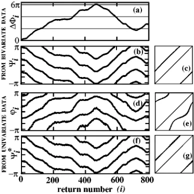
in one direction, i.e., when the phase of oscillations changes by 2. In the absence of noise (D⫽0) a 1:3 phase synchro-nization arises, and is detectable through the associated pla-teau around zero on a⌬⌽(t) plot over the whole observation time; the corresponding map共3兲consists of three points共this case is trivial and is not illustrated here兲. For noise variance D⫽0.15 nonstationary oscillations take place in the system exhibiting epochs of effective 1:3 phase synchronization, which are detectable through the presence of plateaus, and intervals where phase difference slides slowly关Fig. 7共a兲兴.
A phase of forcing at the moments ti, that is relative
phase ⌿i wrapped into the interval 关⫺;兴 is shown
in Fig. 7共b兲. The corresponding circle map is shown in Fig. 7共c兲. Note, that here by construction ⌿˜i⫽⌿i
⫽关⌽f(ti)⫺2i兴 (mod 2)⫽⫺⌬⌽i/3共mod 2兲. In Fig.
7共d兲 the angles i of return times map 关45兴 are shown and their map is given in Fig. 7共e兲.
Next, we analyze the behavior of the system using only univariate data, namely, the variable x(t). From Eq.共8兲the relative phase ⌿i* is reconstructed from angles i whose temporal dependence and map are given in Figs. 7共f兲 and 7共g兲, respectively. Note the remarkable correspondence of Figs. 7共b兲and 7共f兲, and 7共c兲and 7共g兲, which clearly demon-strates that the relation 共8兲still holds even for strongly non-stationary processes. Another significant observation is that maps in Figs. 7共c兲 and 7共g兲, being in fact classical circle maps共compare with Fig. 5兲are very close to being straight lines, thereby confirming that the forcing was indeed weak.
B. Estimation of rotation number from the angles map
In Ref. 关25兴a method was suggested to find the rotation number⫽n/m of synchronization from relative phase⌿i:
the relative phase is extended to the interval 关0;2n兴, the number n being found by trial; once n is found, the number m is given by the number of horizontal stripes in the plot⌿i
versus i. The situation becomes complicated if the process is nonstationary and the transition occurs from synchronization with numerator n1 to that with n2, where n2⫽n2, etc. Then one has to find all possible ni’s by trial and error and to
estimate all the i corresponding to each different epoch of synchronization, which can require time and patience.
But we have shown theoretically in Sec. II C for the ideal stationary noiseless case, and confirmed by simulation in Sec. III A for a nonstationary case, that the relative phase⌿i
can easily be obtained from the angles of return times map, provided that the interaction is weak. Then, in principle, we can apply the already developed technique to the angles and thus estimate the rotation number. However, the angles map has a noticeable advantage over the relative phase, namely, that the shape of a particular angles map is explicitly defined by the value of the rotation number . That means that one can estimate directly from the map without needing to search for the correct value n of the numerator. Equation共10兲 could be used for the ideal noiseless case, which of course does not arise in reality. In real life situations one can esti-mate as an average over some temporal window,
具
典
⫽ 12arccos s
2, s⫽
具
tani⫹coti⫺1典
, 共21兲 where具¯典implies an average over the window. As one re-gime gives way to another, the value of具典changes, respec-tively. [image:8.612.77.271.57.251.2]The rational rotation number n/m describing synchroni-zation should be close to the one defined by Eq.共21兲, which we will further refer to as ‘‘average rotation number,’’ though not precisely equal to it共due to noise and nonstationarity兲. It
FIG. 7. Comparison of different methods to detect phase syn-chronization for a forced Van der Pol system with slowly and ran-domly varying eigenfrequency, Eq.共20兲. Parameter values are given in the text. The first two rows of plots were derived from bivariate data and are 共a兲 the conventional phase difference ⌬⌽i between
response and forcing; 共b兲 relative phase ⌿i; 共c兲 map of relative
phase⌿i⫹1 vs⌿i. The third and fourth rows are obtained from
univariate data:共d兲angles of return times map;共e兲map of angles;
共f兲angles transformed by means of Eq.共8兲;共g兲map of transformed angles. Note the striking similarity of plots共b兲and共f兲, and共c兲and
should be noted that the number of clouds in the angles map does not in general allow one to define the rotation number immediately, because it gives only its denominator m. The same number of clouds m will exist for synchronization with any n, though the clouds will be placed differently. To find the numerator n we suggest finding the approximate rotation number具典using formula共21兲, and then seeking the integer n closest to the value m
具
典
.However, before applying formula共21兲 we should check that it is valid under the circumstances in question, i.e., that the processes under study interact weakly. The most straight-forward way to check this is to obtain the value of具典from Eq.共21兲, to plot the corresponding return function, and to see if it fits experimental map for angles well enough. If it does, we can accept this具典as an approximation of the true rota-tion number; but if not, we cannot rely on the value in question.
There is also a straightforward way to estimate the rota-tion number from the angles i by using its definition 共1兲. However, to do so one needs to be able to extend the discrete angle i in order to make it increase monotonically. In the present paper we use only formula共21兲to estimate the rota-tion number.
The rotation number 具典 for the case of Fig. 7共e兲 is ap-proximated by formula共21兲 as 0.333 27...; the number 3 of parallel stripes in Figs. 7共b兲, 7共d兲, 7共f兲gives the denominator m; and thus the true value of the rotation number correspond-ing to the epochs of phase lockcorrespond-ing is 13. The return function
of map 共11兲 for ⫽1
3 fits the plot in Fig. 7共e兲 with high
accuracy and cannot be distinguished from it, thereby con-firming that the interaction is weak.
C. Three interacting processes
The situation where more than two processes with differ-ent time scales interact is one that is often encountered in complex living systems. We, therefore, consider the case of three interacting processes in systems affected by weak noise, which we will take to be Gaussian. It is clear that the addition of even weak noise will smear the plots in Fig. 6, affecting our ability to detect synchronization between the different processes. However, the extent of the effect will differ for different rhythms. Namely, closed loops as in Fig. 6共d兲 are likely to become hard to distinguish from a large number of discrete points; but we will still observe three isolated clouds of points pointing to synchronization between the basic rhythm and the one with smaller amplitude with rotation number ⫽13. Similarly, the conclusions about the
absence of synchronization between the basic rhythm and those with smaller amplitude as illustrated by Fig. 6共c兲will remain valid even in the presence of noise.
However, noise will definitely prevent one from making judgments about the fine structure of such plots, thus render-ing it almost impossible to establish whether or not the pro-cesses with smaller amplitudes are synchronized with each other. Fluctuational smearing of the plot in Fig. 6共c兲, for example, will prevent one from identifying the number of nonclosed curves共because two of them are likely to merge兲, and smearing of the plot in Fig. 6共d兲 will prevent one from
distinguishing whether each cloud represents a smeared loop or consists of several smeared points.
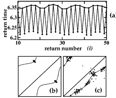
In view of these problems we suggest an extension of our method to remove from consideration the basic rhythm, thereby enabling us to focus our attention on the smaller amplitude processes. Namely, after detecting synchronization or otherwise between the main rhythm and the one of the remaining two, we propose to proceed as follows. Plot the return times Tivs i and form a new dataset consisting of all
their local maxima 共or minima兲as shown in Fig. 8共a兲. Now treat the new data as an independent time series resulting from the interaction of only two processes. One can plot for these data the map of angles and then analyze it by analogy with Sec. III B.
This approach can be realized in application to experi-mental data only in cases where the frequency of the basic process is larger than those of smaller amplitude. However, this condition is often satisfied in practice, as will be illus-trated 关46兴in relation to human heart rate variability data.
To demonstrate the workability of this technique, we ap-ply it to the Van der Pol system forced quasiperiodically and influenced by noise,
x˙⫽y , 共22兲
y˙⫽⑀共1⫺x2兲y⫺0x⫹C1sin⍀1t⫹C2sin⍀2t⫹
冑
D共t兲for ⑀⫽0.1, 0⫽1, C1⫽C2⫽0.1, ⍀1⫽0.5, ⍀2⫽0.1, D
⫽0.000 01. The parameters are selected in such a way that for all the processes effective synchronization takes place, with01⫽
1
2 and12⫽
1
5. In Fig. 8共a兲the sequence of return
times Ti extracted from coordinate y (t), and all its local
maxima, are shown. In Fig. 8共b兲the map for angles is shown for Ti, which consists of two clouds of points共black points兲
lying on a return function 共11兲 for ⫽1
2 共thin black line兲,
being evidence of 1:2 synchronization between the basic
pro-FIG. 8. Quasiperiodically forced Van der Pol system with noise
共22兲. All processes are synchronous. 共a兲 Return times Ti. Local
maxima are connected by a thick solid line. 共b兲,共c兲 Angles-of-return-times map for共b兲Tiand共c兲local maxima of Ti. Thin black
lines show return functions in Eq. 共11兲 for 共b兲 01⫽1/2 共c兲 12
[image:9.612.337.532.57.222.2]cess and the one with frequency ⍀1. At this stage, it is difficult to decide from looking at the map whether or not the smaller amplitude processes are synchronous. Now, plot the map for angles for the set of local maxima of Ti关Fig. 8共c兲兴.
One can clearly distinguish five separate clouds of points here, pointing to synchronization between the processes with small amplitudes, the denominator m of the rotation number being given by the number of clouds. A rough estimate of the rotation number by Eq.共21兲gives 0.212 36 which is close to
1
5共the corresponding return function is shown by a thin black
line兲, and so the correct rotation number of 1
5 has been
suc-cessfuly extracted.
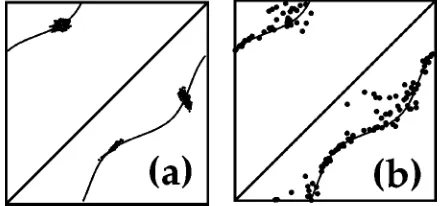
Now, apply our technique to the case when only partial effective synchronization in Eq. 共22兲 takes place. Set ⑀
⫽0.1, 0⫽1, C1⫽0.3, C2⫽0.17, ⍀1⫽0.333 001, ⍀2
⫽0.1001, D⫽0.0001. In Fig. 9共a兲a map for angles of return times is plotted. Three clouds of points testify to the effective 1:3 synchronization between the basic rhythm and forcing with frequency ⍀1. The ‘‘average rotation number’’ calcu-lated from this map by use of Eq.共21兲is 0.333 333, which is a very good approximation of 13. With this, the map for
angles for local maxima of return times shown in Fig. 9共b兲is rather smeared by noise and displays no effective synchroni-zation between forcings. The average rotation number from Eq. 共21兲 is 0.2801 . . . , which is close to the actual frequency ratio of the processes under consideration 12
⫽0.300 599 . . . . The return function for the map共11兲with parameter⫽0.3, shown by a thin black line, seems to fit the map points reasonably well.
Thus, the technique described above seems to be able to provide information about synchronization, or its absence, between each consecutive 共first with second, second with third兲pair of three processes interacting within a nonlinear system, even in the presence of noise.
IV. SUMMARY AND DISCUSSION
To summarize, we have proposed an approach to the de-tection of synchronization 共or the lack of it兲between two or several processes interacting within a single system, using
only a one-dimensional signal coming from it. The approach is based on plotting the map of angles of the return times map, and studying its dynamics. We have revealed an ex-plicit relation between the angles of return times map and the phase difference between interacting processes. The validity of this relation is confirmed also for nonstationary processes in a model.
Explicit maps have been derived describing the behavior of the angles-of-return-times map for a system with a limit cycle forced by an arbitrary number of harmonic signals of small amplitude. The maps obtained appear to describe well numerically simulated data under appropriate conditions.
All the formulas describing the angles’ behavior can be derived not only for the return times map, but also for the stroboscopic map reconstructed from a one-dimensional sig-nal by the delay method. Moreover, as numerical simulations have shown, they also fit well angles of Poincare´ sections reconstructed from one-dimensional time series. The reason for presenting the above discussion in relation to the return times map, rather than for the stroboscopic map, comes back to the reason for writing this paper: to obtain a stroboscopic section we would need to link ourselves to an external forc-ing, or to a signal from interacting partial subsystem, and these are by definition absent or unknown in the context of the problem posed.
Although the same 共or similar兲 formulas should in prin-ciple be obtainable for the reconstructed Poincare´ map within the framework of our starting suppositions 共4兲,共15兲, we failed to do so because of the complicated transcendental equations that arise.
Given a one-dimensional time series, we can find the map for angles by reconstructing either the Poincare´ or the return times map. Both of these operations seems equally valid and should lead to the same results for dynamical systems. How-ever, in practice, data from medical or biological experi-ments are often already presented in the form of return times, like R-R intervals of human electrocardiogram. Moreover, the algorithm for extraction of return times can be simpler than that for the Poincare´ section, the latter being connected with restoration of the phase portrait in a multidimensional phase space and searching for intersection of the phase tra-jectory with a secant hypersurface. Of course, one should decide for oneself which method is preferable in any particu-lar case.
V. CONCLUSIONS
Based on the results presented above, we arrive at the following conclusions.
For two weakly interacting processes, the angles of return times map can be transformed to a relative phase by means of Eq.共8兲.
[image:10.612.64.284.59.162.2]Without noise, when a weak periodic forcing is applied to a periodic oscillator, the dynamics of angles of return times does not depend on the amplitude of forcing and is com-pletely defined by the rotation number. When a periodic os-cillator is forced quasiperiodically and weakly, the dynamics of angles is defined not only by partial rotation numbers, but also by the ratios of the forcing amplitudes.
FIG. 9. Quasiperiodically forced Van der Pol system with noise
共22兲. The basic process is synchronous with that with ⍀2. The
process with⍀3is not synchronous with either of the other two.共a兲
Angles map for return times map.共b兲Angles map for local maxima of return times. The thin black lines show return functions of Eq.
The technique of eliminating the higher-frequency com-ponents by extracting local extrema from the return times allows one to reach a judgment about the synchronization or otherwise of each successive pair of processes involved, for at least three processes.
We, therefore, expect that the proposed approach is likely to be useful in application to the analysis of different kinds of real data, for example, biological. It is applied to heart rate variability data in the paper关46兴that follows.
ACKNOWLEDGMENTS
We are much indebted to Dr. Alexander Neiman for valu-able discussions and for his constructive comments on a draft version of the manuscript. The work was supported by the Engineering and Physical Sciences Research Council 共UK兲, the Leverhulme Trust, the Medical Research Council 共UK兲, and the U.S. Civilian Research Development Foundation 共Award No. REC 006兲.
关1兴B. Van der Pol, Radio Rev. 1, 704共1920兲.
关2兴V. I. Arnold, Complementary Chapters of Ordinary Differen-tial Equation Theory共Nauka, Moscow, 1978兲.
关3兴A. N. Malakhov, Fluctuations in Self-Oscillatory Systems 共Nauka, Moscow, 1968兲 共in Russian兲.
关4兴R. L. Stratonovich, Topics in Theory of Random Noise共 Gor-don and Breach, New York, 1963兲.
关5兴C. Hayashi, Nonlinear Oscillations in Physical Systems 共McGraw-Hill, New York, 1964兲; I. I. Blekhman, Synchroni-zation in Science and Technology 共ASME Press, New York, 1988兲.
关6兴Yo. Kuramoto, Prog. Theor. Phys. Suppl. 79, 223共1984兲. 关7兴V. S. Afraimovich, N. N. Verichev, and M. I. Rabinovich, Izv.
VUZov, Radiofiz. 29, 1050共1989兲.
关8兴L. M. Pecora and T. L. Carroll, Phys. Rev. Lett. 64, 821 共1990兲.
关9兴V. S. Anishchenko, T. E. Vadivasova, D. E. Postnov, and M. A. Safonova, Radiotekh. Elektron.共Moscow兲36, 338共1991兲; Int. J. Bifurcation Chaos Appl. Sci. Eng. 2, 633共1992兲.
关10兴M. Rosenblum, A. Pikovsky and J. Kurths, Phys. Rev. Lett. 76, 1804共1996兲; A. S. Pikovsky, M. G. Rosenblum, G. V. Osipov, and J. Kurths, Physica D 104, 219共1997兲.
关11兴A. Neiman, A. Silchenko, V. S. Anishchenko and L. Schimansky-Geier, Phys. Rev. E 58, 7118共1998兲.
关12兴A. Neiman, Phys. Rev. E 49, 3484共1994兲.
关13兴A. Silchenko, T. Kapitaniak, and V. S. Anishchenko, Phys. Rev. E 59, 1593共1999兲.
关14兴B. Shulgin, A. Neiman, and V. Anishchenko, Phys. Rev. Lett. 75, 4157共1995兲.
关15兴S. K. Han, T. G. Yim, D. Postnov, and O. Sosnovtseva, Phys. Rev. Lett. 83, 1771共1999兲.
关16兴V. S. Anishchenko, A. G. Balanov, N. B. Janson, N. B. Igo-sheva, and G. V. Bordyugov, Int. J. Bifurcation Chaos Appl. Sci. Eng. 10, 2339共2000兲.
关17兴N. F. Rulkov, Chaos 6, 262共1996兲.
关18兴P. Tass, M. G. Rosenblum, J. Weule, J. Kurths, A. Pikovsky, J. Volkmann, A. Schnitzler, and H.-J. Freund, Phys. Rev. Lett. 81, 3291共1998兲.
关19兴R. C. Elson, A. I. Selverston, R. Huerta, N. F. Rulkov, M. I. Rabinovich, and H. D. I. Abarbanel, Phys. Rev. Lett. 81, 5692 共1998兲.
关20兴A. Neiman, Xing Pei, D. Russell, W. Wojtenek, L. Wilkens, F. Moss, H. A. Braun, M. T. Huber, and K. Voigt, Phys. Rev. Lett. 82, 660共1999兲.
关21兴G. Matsumoto, K. Aihara, Y. Hanyu, N. Takahashi, S.
Yoshizava, and J. Nagumo, Phys. Lett. A 123, 162共1987兲. 关22兴J. Sturis, C. Knudsen, N. M. O’Meara, J. S. Thomsen, E.
Mosekilde, E. Van Cauter, and K. S. Polonsky, Chaos 5, 193 共1995兲.
关23兴M. Santini, C. Pandozi, F. Colivicchi, F. Ammirati, M. Carmela Scianaro, A. Castro, and F. Lamberti, G. Gentilucci, Eur. Heart J. 21, 848共2000兲; G. Leblanc, C. Michel, P. Y. Laffy, F. Mer-cier, and J. N. Fabiani, Cardiovasc. Surg. 5, S8共1997兲. 关24兴M. Schiek et al., in Nonlinear Analysis of Physiological Data,
edited by H. Kantz, J. Kurths, and G. Mayer-Kress共Springer, Berlin, 1998兲.
关25兴C. Scha¨fer, M. G. Rosenblum, J. Kurths, and H.-H. Abel, Na-ture共London兲392, 239共1998兲.
关26兴Milan Palus and Dirk Hoyer, IEEE Eng. Med. Biol. Mag. 17, 40共1998兲.
关27兴A. Stefanovska and M. Bracˇicˇ, Contemp. Phys. 40, 31共1999兲. 关28兴A. Stefanovska, H. Haken, P. V. E. McClintock, M. Hozˇicˇ, F.
Bajrovic´, and S. Ribaricˇ, Phys. Rev. Lett. 85, 4831共2000兲. 关29兴H. Bettermann, D. Amponsah, D. Cysarz, and P. Van Leeuwen,
Am. J. Physiol. 277, H1762共1999兲.
关30兴A. Stefanovska and M. Hozˇicˇ, Prog. Theor. Phys. Suppl. 139, 270共2000兲.
关31兴N. B. Janson, A. G. Balanov, V. S. Anishchenko, and P. V. E. McClintock, Phys. Rev. Lett. 86, 1749共2001兲.
关32兴F. Takens, in Dynamical Systems and Turbulence, Warwick, 1980, edited by D. A. Rang and L. S. Young, Lecture Notes in Mathematics Vol. 898共Springer, Berlin, 1981兲, p. 366. 关33兴J. Stark, D. S. Broomhead, M. E. Davies, and J. Huke,
Non-linear Anal., Theory, Methods Appl. 30, 5303共1997兲. 关34兴R. Hegger and H. Kantz, Europhys. Lett. 38, 267共1997兲. 关35兴N. B. Janson, A. N. Pavlov, A. B. Neiman, and V. S.
Anish-chenko, Phys. Rev. E 58, R4共1998兲.
关36兴H. Herzel, H. Seidel, and H. Warzel, Wiss Z. Humboldt Univ. Berl.关Reihe Medizin兴41, 51共1992兲.
关37兴K. Suder, F. R. Drepper, M. Schiek, and H.-H. Abel, Model. Physiol. 44, H1092共1998兲.
关38兴J. Godelle and C. Letellier, Phys. Rev. E 62, 7973共2000兲. 关39兴The same expressions 共10兲 and 共11兲 can be obtained for the
return times map constructed from the time moments when the function y (t)⫽x˙(t) takes zero values, and also for the strobo-scopic section of signal x(t) obtained by delay reconstruction from the values xi⫽x(关2/⍀兴i) taken over complete periods
关40兴O. E. Ro¨ssler, Phys. Lett. 57A, 397共1976兲.
关41兴T. E. Vadivasova, A. G. Balanov, O. V. Sosnovtseva, D. E. Postnov, and E. Mosekilde, Phys. Lett. A 253, 66共1999兲. 关42兴V. I. Arnol’d, Geometrical Methods in the Theory of Ordinary
Differential Equations 共Springer-Verlag, New York, 1983兲; J. Guckenheimer and P. Holmes, Nonlinear Oscillations, Dy-namical Systems and Bifurcations of Vector Fields 共 Springer-Verlag, New York, 1983兲; L. Glass, Chaos 1, 13共1991兲. 关43兴If two processes are synchronized, but the strength of
interac-tion is large, one cannot use the map共11兲 to describe the dy-namics of angles. However, the resulting signal can still be approximated by a sum of several most significant sine terms
with frequencies , 2,...,⍀, 2⍀,...,⫾⍀, ⫾2⍀,..., etc. Then the map共18兲can reliably describe the behavior of angles. 关44兴S. Newhouse, D. Ruelle, and F. Takens, Commun. Math. Phys.
64, 35共1979兲.
关45兴Since the process is substantially nonstationary, return times oscillate around an average value that is floating randomly. Before extracting angles, this floating average was removed by the technique of derivatives described in Ref.关46兴.