VISION-BASED OBSTACLE AVOIDANCE FOR A SMALL,
LOW-COST ROBOT
Chau Nguyen Viet, Ian Marshall
Computer Science Department, University of Kent, Canterbury, United Kingdom [email protected], [email protected]
Keywords: obstacle-avoidance, robot vision.
Abstract: This paper presents a vision-based obstacle avoidance algorithm for a small indoor mobile robot built from low-cost, and off-the-shelf electronics. The obstacle avoidance problem in robotics has been researched ex-tensively and there are many well established algorithms for this problem. However, most of these algorithms are developed for large robots with expensive, specialised sensors, and powerful computing platforms. We have developed an algorithm that can be implemented on very small robots with low-cost electronics and small computing platforms. Our vision-based obstacle detection algorithm is fast and works with very low resolution images. The control mechanism utilises both visual information and sonar sensor’s measurement without having to fuse the data into a model or common representation. The robot platform was tested in an unstructured office environment and demonstrated a reliable obstacle avoidance behaviour.
1
INTRODUCTION
Autonomous navigation in an unstructured envi-ronment, i.e. an environment that is not modified specifically to suit the robot, is a very challenging task. Current robots that can operate autonomously in an unmodified environment are often large and ex-pensive. Most of today robot navigation algorithms rely on heavy and power-hungry sensors such as laser range finders, high resolution stereo-visions (Thrun et al., 1999; Manduchi et al., 2005; Stentz et al., 2003; Ibanez-Guzman et al., 2004; Batalin et al., 2003). As a consequence, these robots require powerful comput-ing units to be mounted on-board. The size, com-putational power, and energy requirements of these robots limit the range of their applications and opera-tional period. In this work, we have built a small mo-bile robot from cheap off-the-self electronics to per-form obstacle avoidance in an unstructured environ-ment. Obstacle avoidance is the first basic behaviour needed for an autonomous mobile robot. The robot is equipped with a low-power camera and two ultra-sonic sensors. Image processing is done in real-time and on-board. Our robot is small and energy efficient; it is powered by AA batteries.
Obstacle avoidance is one of the most fundamen-tal and researched problems in the field of mobile robotics. Most obstacle avoidance algorithms uses active range sensors such as ultrasonic sensors, laser range finders and infra-red sensors. Visual sensors are an alternative solution for obstacle avoidance and becoming increasingly popular in robotics. Visual sensors often provides better resolution data, longer ranges at faster rates than range sensors. Because vi-sual sensors are inactive they are less dependent on the environment. However image processing is a very computationally expensive task. Vision often require complicated software and powerful computing plat-form or dedicated hardware module. For very small robots, i.e. those that are man-carriable, vision is still rare.
extracted from a sequence of images from a single camera using motion parallax (Lu et al., 2004). This technique was used for obstacle avoidance in (Santos-Victor et al., 1993; Zufferey and Floreano, 2005). For the output of this algorithm to be accurate, the im-age processing rate must be high enough e.g. over 30 frames per second. Another class of algorithm is based on colour-based terrain segmentation (Lorigo et al., 1997; Lenser and Veloso, 2003; Ulrich and Nourbakhsh, 2000). This approach works on a sin-gle image. If we can assume the robot is operating on a flat surface and all objects have their bases on the ground, the distance from the robot to an object is linear to the y-axis coordinate of the object in the perceived image. The problem is reduced to classi-fying a pixel into two classes, obstacle or traversable ground. This approach is suitable for robots that oper-ate indoor or on benign flat terrains. Since it does not requires high resolution images or high frame rates camera, we adopt this approach for our vision mod-ule. What makes our algorithm different from exist-ing algorithms is the use of a lookup map for colour classification and a reduced colour space. Lookup map is a very fast classification method. On a Gum-stix computer clocks at 200 MHz, our algorithm can process more than 500 frames of 87∗44 pixels per
second. The vision algorithm presented in (Lenser and Veloso, 2003) uses 3 array access operations and an AND bitwise operations for each pixel. Our al-gorithm uses only one array access operation. Lug-ino and her group developed an algorithm that can work with low resolution image 64*64 pixels frame in (Lorigo et al., 1997). Our algorithm works with even use lower resolution image of 22*30 pixels frame. This reduces the computing cycle required for the vi-sion algorithm and enable our algorithm to run on em-bedded computing devices.
Although our vision algorithm is reliable, due to hardware limitation, the camera we uses has a nar-row field of view (FOV), two additional sonar sen-sors were added to expand the robot’s FOV. This does not conflict with our preference of vision sensor over range sensor. Vision is the main sensor and the sonar sensors were added to improve the performance of the system only. The control mechanism is reactive, it has no memory and acts upon the most current sen-sor readings only. This allows the robot responds quickly to changes in the environment. While many other systems fuse data from different sensor sources into a single representation or world model, our algo-rithm does not. There is no attempt to fuse distance estimates from visual images and sonar sensors into any kind of model or representation. Instead, the con-trol rules are tightly coupled with sensory data and
the hardware configuration. This gives rise to a fast and robust obstacle avoidance behaviour. Our robot is able to response to changes in the environment in real-time. The approach we used is inspired by the subsumption architecture (Brooks, 1985) and Brain-tenberg vehicles (BraiBrain-tenberg, 1984).
Our main contribution is an obstacle avoidance al-gorithms that uses low-power off-the-self camera and runs on a small constrained platform. Even with very low resolution colour images our robot demonstrates a robust obstacle avoidance behaviour. The robot was tested in a real office environment and was shown to be very robust; the robot could operate autonomously over a long period of time. This work emphasised the efficiency and simplicity of the system. We want to build an autonomous robot with the minimal hard-ware configuration. We implemented the controller on the Gumstix Linux computer, which runs at 200 MHz. But the algorithm can run on a slower micro-processor as it uses only a small fraction of the Gum-stix’s processing cycle. The obstacle avoidance algo-rithm might be used as a module in a more complex system e.g. the first level of competence in a sub-sumption architecture. It can be used on it own in an application such as exploration, surveillance. Be-cause only a small fraction of the CPU is required for obstacle avoidance, more spaces are available for more complex behaviours on the platform.
This paper is organised as follows. In section II, we present the vision algorithm and control mecha-nism. Section III describes the hardware configura-tion and software implementaconfigura-tion. The experiments and results are reported in section IV. In section V, we conclude with some remarks and our future plan.
2
Vision and Control Algorithm
2.1
Ground and obstacles segmentation
In our classification algorithm, pixels are classified according to their colour appearance only. The colour space we use is the RGB colour space. Each colour in the colour space is set to be a ground or obsta-cle colour. This classification information is stored in a binary lookup map. The map is implemented as a three dimensions vector of integers. To classify a pixel, its RGB components are used as indices to ac-cess the class type of the pixel. The classification pro-cess is very fast since for each pixel only one array lookup operation is needed.
number of pixels of each colour in the example pic-tures. Then if the number of pixels of a colour is more than 5% of the total number of pixels in those pictures, that colour is set to be a ground colour. The 5% threshold is used to eliminate the noises in the im-ages. Procedure 1 describes this calibration process. A lookup map is also very efficient for modification. At the moment, the calibration process is done once before the robot starts moving and the lookup map remains unchanged. We anticipate that the colour ap-pearance of the ground and the lightning condition are likely to change if the robot operates for a long pe-riod or moves into different environments and there-fore any classification technique is required to adapt to these changes. In the near future, we plan to im-plement an on-line auto-calibrating algorithm for the vision module. Procedure 2 describes how a pixel is classified during the robot’s operation.
The main drawback of using the lookup map is memory usage inefficiency. In a constrained platform the amount of memory needed to store the full 24 bits RGB space is not available. To overcome this prob-lem, we reduce the original 24 bits RGB colour space to 12 bits and decrease the size of lookup table from 224 elements to 212 elements. Effectively, we lower the resolution of the colour space but also make the classifier more general since each element of the re-duced table represents a group of similar colours in the original space. We also use very low resolution images of 22∗30 pixles. Fig. 1 has two examples
of the outputs from this segmentation procedure. At the top row, there is a picture taken from the cam-era mounted on our robot at maximum resolution and the binary image produced by the segmentation pro-cedure. The binary image contains some noise and a falsely classifies a part of a box as ground since their colours are similar. Nevertheless in this case, the dis-tance to the box’s base is still correctly measured. At the bottom row is the down-sampling version of the top row picture and its corresponding binary image.
The output of the image segmentation is a binary image differentiating obstacles from the ground. As-suming all objects have their bases on the ground, the distance to an object is the distance to its base. This distance is linear to the y-coordinate of the edge be-tween the object and the floor in the binary image. For obstacle avoidance, we only need the distance and width of obstacles but not their height and depth. Therefore a vector of distances to the nearest obsta-cles is sufficient, we call this obstacle distance vector (ODV). We convert the binary image to the required vector by copying the lowest y-coordinate of a non-floor pixel in each column to the corresponding cell in the vector. Each element of the vector represents
the distance to the nearest obstacle in a specific direc-tion.
Procedure 1 PopulateLookupMap ( n: number of
pixels , P : array of n pixels
for i=0 to n−1 do
(R,G,B) =⇐rescale(P[i]r,P[i]g,P[i]b)
pixel counter[R][G][B] ⇐
pixel counter[R][G][B] +1
end for
for (R,G,B) = (0,0,0) to MAX(R,G,B) do
is ground map[R][G][B] ⇐
pixel counter[R][G][B]>n∗5% end for
return is ground map
Procedure 2 is ground(p : pixel )
(R,G,B)⇐rescale(pr,pg,pb) return is ground map[R][G][B];
2.2
Control algorithm
The control algorithm we adopted is reactive. Deci-sions are made upon the most recent sensory readings. The inputs to the controller are the obstacle distance vector, produced by the visual module, and distance measurements from two sonar sensors pointing at the sides of the robot. The ODV gives a good resolution distance map of any obstacle in front of the robot. Each cell in the vector is the distance to the nearest obstacle in a direction of an angle of about 2.5◦
. The angular resolution of the two sonar sensors are much lower. So the robot has a good resolution view at the front and lower at the sides. The controlling mecha-nism consists of several reflexive rules.
• If there are no obstacles detected in the area
mon-itored by the camera, run at maximum speed.
• If there are objects in front but further than the
trigger distance, slow down.
• If there are objects within the trigger distance,
start to turn to an open space.
• If a sonar sensor reports a very close object, within
5 cm, turn to the opposite direction.
C
B
[image:4.612.116.481.88.367.2]D A
Figure 1: The images processed by the vision module. A is a full resolution colour image. B is the binary obstacle-ground image of A. C is a low resolution image from A and D is its corresponding binary image
there are obstacles in both left and right half of the image, the two measurements from sonar sensors are compared and the robot will turn to the direction of the sonar sensor that reports no existence of obstacles or a biger distance measurement. There is no attempt to incorporate or fuse data from the camera and sonar sensors together into a uniformed representation. The algorithm uses the sensor readings as they are.
3
Platform Configuration And
Implementation
The robot control software runs on the Gumstix (gum, ), a small Linux computer that has an Intel 200 MHz ARM processor with 64 Mb of RAM. The vision sensor is a CMUcam2 module connected to the Gumstix via a RS232 link. A Brainstem micro-controller is used to control sonar sensors and servos. The robot is driven by two servos. These electronic devices are mounted on a small three wheeled robot chassis. The total cost of all the components is less than 300 US dollars. The robot can turn on the spot with a small radius of about 5 cm. Its maximum speed is 15cm/s. The robot is powered by 12 AA batteries. A fully charged set of batteries can last for up to 4
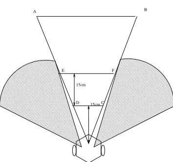
hours. Fig. 2 shows the area in front of the robot that is monitored by the robot’s sensors. The CMUcam is mounted on the robot pointing forward at horizontal level and captures an area of about 75cm2. Because the camera has a relatively narrow FOV of about 55◦
, the two sonar sensors on the side are needed. In total, the robot’s angle of view is 120◦
. The robots dimen-sions are 20cm∗20cm∗15cm. The hardware
config-uration was determined by the trial and error method. The parameters we presented here were the best that we found and were used in the experiments reported in section IV.
The maximum frame resolution of the CMUCam2 is 87∗144 pixels, we lower the resolution to only
22∗30 pixels. We only need the first bottom half
of the picture so the final image has dimensions of 22∗15. The resolution down-sampling and picture
cropping is done by the CMUcam module, only the final images are sent to the control algorithm running on the Gumstix.
In our implementation, the obstacle distance vec-tor has 22 cells, each cell corresponds to an angle of 2.5◦
0000000000 0000000000 0000000000 0000000000 0000000000 0000000000 0000000000 0000000000 0000000000 0000000000 0000000000 0000000000 0000000000 0000000000 0000000000 0000000000 0000000000 0000000000 1111111111 1111111111 1111111111 1111111111 1111111111 1111111111 1111111111 1111111111 1111111111 1111111111 1111111111 1111111111 1111111111 1111111111 1111111111 1111111111 1111111111 1111111111 00000000000000 00000000000000 00000000000000 00000000000000 00000000000000 00000000000000 00000000000000 00000000000000 00000000000000 00000000000000 00000000000000 00000000000000 00000000000000 00000000000000 00000000000000 00000000000000 00000000000000 00000000000000 00000000000000 00000000000000 00000000000000 00000000000000 00000000000000 00000000000000 00000000000000 00000000000000 00000000000000 00000000000000 00000000000000 00000000000000 00000000000000 00000000000000 00000000000000 11111111111111 11111111111111 11111111111111 11111111111111 11111111111111 11111111111111 11111111111111 11111111111111 11111111111111 11111111111111 11111111111111 11111111111111 11111111111111 11111111111111 11111111111111 11111111111111 11111111111111 11111111111111 11111111111111 11111111111111 11111111111111 11111111111111 11111111111111 11111111111111 11111111111111 11111111111111 11111111111111 11111111111111 11111111111111 11111111111111 11111111111111 11111111111111 11111111111111 00000000000 00000000000 00000000000 00000000000 00000000000 00000000000 00000000000 00000000000 00000000000 00000000000 00000000000 00000000000 00000000000 00000000000 00000000000 00000000000 00000000000 11111111111 11111111111 11111111111 11111111111 11111111111 11111111111 11111111111 11111111111 11111111111 11111111111 11111111111 11111111111 11111111111 11111111111 11111111111 11111111111 11111111111 0000000000000000 0000000000000000 0000000000000000 0000000000000000 0000000000000000 0000000000000000 0000000000000000 0000000000000000 0000000000000000 0000000000000000 0000000000000000 0000000000000000 0000000000000000 0000000000000000 0000000000000000 0000000000000000 0000000000000000 0000000000000000 0000000000000000 0000000000000000 0000000000000000 0000000000000000 0000000000000000 0000000000000000 0000000000000000 0000000000000000 0000000000000000 0000000000000000 0000000000000000 0000000000000000 0000000000000000 0000000000000000 1111111111111111 1111111111111111 1111111111111111 1111111111111111 1111111111111111 1111111111111111 1111111111111111 1111111111111111 1111111111111111 1111111111111111 1111111111111111 1111111111111111 1111111111111111 1111111111111111 1111111111111111 1111111111111111 1111111111111111 1111111111111111 1111111111111111 1111111111111111 1111111111111111 1111111111111111 1111111111111111 1111111111111111 1111111111111111 1111111111111111 1111111111111111 1111111111111111 1111111111111111 1111111111111111 1111111111111111 1111111111111111 15cm 15cm A B D C E F
Figure 2: A visualisation of the monitored area. ABCD : the area captured by the camera. Shaded areas represent the sonar sensors views. Segment EF is the trigger distance line
the resolution of the images is very low, the distance estimation is not very accurate. At the lowest row of the image, where the ratio between pixel and the pro-jected real world area is highest, each pixel represents an area of 2∗1.5cm2.
The distance that triggers the robot to turn is set to 30 cm. The robot needs to turn fast enough so that the object will not be closer than 15 cm in front of it since the distance of any object in this area can not be cal-culated correctly. At maximum speed , the robot will have about two seconds to react and if the robot has already slowed down while approaching the object, it will have about three seconds. We have tried many different combinations of trigger distances and turn-ing speeds to achieve a desirable combination. The first criteria is that the robot must travel safely, this criteria sets the minimum turning speed and distance. The width of view of the camera at the distance of 30 cm from the robot or 35 cm from the camera is 30 cm. The width of our robot is 20 cm, so if the vi-sion module does not find an obstacle inside the trig-ger range, the robot can safely move forward. The second criteria is the robot needs to be able to go to cluttered areas. This means it should not turn too early when approaching objects. Also when the robot is confronted by the wall or a large object, it should turn just enough to move along the wall/object and not bounce back. This criteria encourages the robot to explore the environment.
The main drawback of the no map approach is that the robot might get stuck in a confined or looped area. A common solution and opposite to ours is to build a model of the environment surrounding the robot. The model is a global map and can be used for planning a desirable path. Also the model can give the robot a
virtual wider angle field of view by remembering ob-jects that a robot saw from the previous experience. However with our robot configuration, the reactive mechanism can solve this problem. Since the robot can turn on the spot, we can guarantee that the robot will not be trapped indefinitely.
4
Experiments
4.1
Experiment Setup and Results
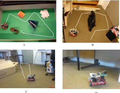
We tested the robot in two environments, a 1.5∗2.5m2
artificial arena surrounded by 30cm height walls and an office at the University of Kent Computing de-partment, shown in Fig. 3. The surface of the arti-ficial arena is a flat cartoon board with green wall-papers on top. We put different real objects such as boxes, shoes, books onto the arena. We first tested the robot in the arena with no objects (the only obstacless are walls) and then made the tests more difficult by adding objects. The office is covered with a carpet. The arena presents a more controlable environment where the surface is smooth and relatively colour-uniformed. The office environmnent is more chal-lenging where even though the ground is flat its sur-face is much more coarse and not colour-uniformed.
For each test, the robot run for 5 mins. We placed the robot in different places and put different objects into the test area. In general, the robot is quite compe-tent; Table I summaries the result. The vision-based obstacle detection module correctly identified obsta-cle with almost 100% accuracy, that is if there was an obstacle in the camera view, the algorithm would reg-ister an non-ground area. Although the calculated dis-tances of obstacles are not very accurate, they provide enough information for the controller to react. The simple mechanism of finding an open space worked surprisingly well. The robot was good at finding a way out in a small area such as the areas under tables and between chairs. The number of false positives are also low and only occured in the office environment. This is because the office’s floor colours are more dif-ficult to capture thoroughly. Further analysis revealed that false positives often occurred in the top part of the images. This is explained by the ratio of pixels/area in the upper part of the image being lower than the bottom part. At the top row of the image, each pixel corresponds to an area of 7∗4cm while at the
bot-tom row the area is 2∗1.5cm. Fortunately, the upper
capa-A B
C D
[image:6.612.97.498.140.449.2]Figure 3: Snapshots of the robot in the test environments and its trajectories. A: the artificial arena with 4 objects. B: A small area near the office corner. C: A path that went through a chair’s legs. D: An object with no base on the ground.
Table 1: Performance summary
Environment No of Obstacles Duration Average speed No. of collisions False positive
Arena 0 60 min 13 cm/c 0 0%
Arena 1 60 min 10 cm/s 0 0%
Arena 4 60 min 6 cm/s 2 0%
ble of responding quickly to changes in the environ-ments. During some of the tests, we removed and put obstacles in front of the robot. The robot can instantly recognise the changes and changed it’s course accord-ingly.
There are a small number of cases where the robot collided. Most of the collisions occurred when there are close objects in the direction that the robot was turning into and the sonar sensor failed to report the obstacles. Also there are objects that do not have their bases on the ground for the robot to see, in those sit-uations there were miscalculations of the distances to the objects and hence collisions. In our environment, one of the objects that presented this problem was ta-ble cross-bar, ( Fig. 3 D )
Fig. 3 shows 4 snapshots of the robot during op-eration and its trajectory. In picture A, the robot ran in the arena with 4 obstacles, it successfully avoided all the objects. On picture B, the robot went into a small area near a corner with a couple of obstacles and found a way out. On picture C, the robot success-fully navigated through a chair’s legs which presented a difficult situation. Picture D was a case where the robot failed to avoid an obstacle. Because the table leg cross-bar is off the floor, the robot underestimated the distance to the bar.
4.2
Discussion
We found that adding more obstacles onto the arena did not make the number of collisions increase sig-nificantly. However the average speed of the robot dropped as the arena get more crowded. The speed loss is admitedly due to the robot’s reactive behaviour. The robot does not have a path planning therefore it can not always select the best path and only reacts to the current situation. In some cluttered areas, the robot spent a lot of time spinning around before it can find a viable path. We can improve the robot’s behaviour in these situations by having a mechanism to detect cluttered and closed areas so the robot can avoid them. The assumption that the travelling sur-face is flat holds for most indoor environments. How-ever, there a few objects that do not have their bases on the ground or protrude from their bases. Another sonar sensor pointing at the front of the robot will solve this problem. The additional sensor can also be used for auto-calibarating the vision module.
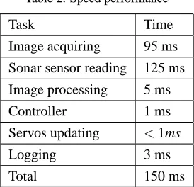
Each control cycle takes about 150ms or 7Hz. Ta-ble II shows the time spent on each task in the cycle. Most of the times is spent waiting for the camera im-ages and sonar data. The algorithm used only 15% of the CPU during operation. This leaves plenty of resources for higher behaviours if needed. It is
possi-Table 2: Speed performance
Task Time
Image acquiring 95 ms
Sonar sensor reading 125 ms
Image processing 5 ms
Controller 1 ms
Servos updating <1ms
Logging 3 ms
Total 150 ms
ble to implement this algorithm with a less powerful CPU. Since only 10% of the CPU time is spent on processing data, a CPU running at 20 MHz would be sufficient. So instead of the Gumstix computer we can use a micro-controller such as a Brainstem or a BA-SIC STAMP for both image processing and motion control without any decrease in performance. The memory usage is nearly one Mb which is rather big. We did not try to optimise memory usage while im-plementing the code so improvements could be made. We plan to implement this control algorithm on a micro-controller instead of the Gumstix. This change will reduce the cost and power usage of the robot by a large amount. To the best of our knowledge, there has not been a mobile robot that can perform reliable obstacle avoidance in unconstrained environ-ments using such low resolution vision and slow mi-croprocessor. A robot with only obstacle avoidance behaviour might not be very useful apart from appli-cations such as exploration or surveillance. However given that our algorithm is very computationally ef-ficient and requires low resolution images, it can be incorporate into a more complex system at a small price and leaves plenty of resources for higher level behaviours.
5
Conclusion and future research
[image:7.612.347.484.104.236.2]in-stead the controller only reacts to immediate sensor measurements. The obstacle avoidance strategy is de-rived from the combination of the robot’s dynamics and sensor setting. The robot was tested in a real of-fice environment and performed very well.
One of the biggest disadvantages of colour-based object detection is the need of calibrating the vision module before operation. It is very desirable to have a robot that can be deployed in any environment that meets some specific requirements without prepara-tion. We are implementing a simple auto-calibrating procedure on-board the robot. This procedure will be run before each operation. The robot must be de-ployed in a place where the immediate area in front of it is free of obstacles. The robot will move forward for a few seconds and take pictures of the floor for the calibration process. Another approach is to add an-other sonar sensor pointing forward with the camera. The correlation between this sonar measurement and the visual module output can be learned. This corre-lation then can be used for auto-calibrating the visual module.
REFERENCES
http://www.gumstix.org.
Batalin, M., Shukhatme, G., and Hattig, M. (2003). Mobile robot navigation using a sensor network. IEEE International Conference on Robotics & Automation (ICRA), 2003.
Braitenberg, V. (1984). Vehicles: Experiments in Syn-thetic Psychology. MIT Press/Bradford books.
Brooks, R. A. (1985). A robust layered control sys-tem for a mobile robot. Technical report, MIT, Cambridge, MA, USA.
Ibanez-Guzman, J., Jian, X., Malcolm, A., Gong, Z., Chan, C. W., and Tay, A. (2004). Autonomous armoured logistics carrier for natural environ-ments. In Intelligent Robots and Systems, 2004. (IROS 2004). Proceedings. 2004 IEEE/RSJ In-ternational Conference on, volume 1, pages 473–478.
Lenser, S. and Veloso, M. (2003). Visual sonar: fast obstacle avoidance using monocular vision. In Intelligent Robots and Systems, 2003. (IROS 2003). Proceedings. 2003 IEEE/RSJ Interna-tional Conference on, volume 1, pages 886–891.
Lorigo, L., Brooks, R., and Grimsou, W. (1997). Visually-guided obstacle avoidance in unstruc-tured environments. In Intelligent Robots and Systems, 1997. IROS ’97., Proceedings of the
1997 IEEE/RSJ International Conference on, volume 1, pages 373–379, Grenoble, France.
Lu, Y., Zhang, J., Wu, Q., and Li, Z.-N. (2004). A survey of motion-parallax-based 3-d reconstruc-tion algorithms. Systems, Man and Cybernetics, Part C, IEEE Transactions on, 34(4):532–548.
Manduchi, R., Castano, A., Talukder, A., and Matthies, L. (2005). Obstacle detection and ter-rain classification for autonomous off-road navi-gation. Autonomous Robot, 18:81–102.
Santos-Victor, J., Sandini, G., Curotto, F., and Garibaldi, S. (1993). Divergent stereo for robot navigation: learning from bees. In Computer Vi-sion and Pattern Recognition, 1993. Proceedings CVPR ’93., 1993 IEEE Computer Society Con-ference on, pages 434–439, New York, NY.
Stentz, A., Kelly, A., Rander, P., Herman, H., Amidi, O., Mandelbaum, R., Salgian, G., and Pedersen, J. (2003). Real-time, multi-perspective percep-tion for unmanned ground vehicles. AUVSI.
Thrun, S., Bennewitz, M., Burgard, W., Cremers, A., Dellaert, F., Fox, D., Hahnel, D., Rosenberg, C., Roy, N., Schulte, J., and Schulz, D. (1999). MINERVA: a second-generation museum tour-guide robot. In Robotics and Automation, 1999. Proceedings. 1999 IEEE International Confer-ence on, volume 3, pages 1999–2005, Detroit, MI, USA.
Ulrich, I. and Nourbakhsh, I. R. (2000). Appearance-based obstacle detection with monocular color vision. In AAAI/IAAI, pages 866–871.