The Mean Residual Lifetime of (n － k + 1) out of n Systems in Discrete Setting

http://dx.doi.org/10.4236/am.2014.53046

The Mean Residual Lifetime of (n

−

k + 1)-out-of-n

Systems in Discrete Setting

Maryam Torabi Siahboomi

Department of Statistics, Science and Research branch, Islamic Azad University, Tehran, Iran Email: m.torabi@mau.ac.ir

Received November 2, 2013; revised December 2, 2013; accepted December 9,2013

Copyright © 2014 Maryam Torabi Siahboomi. This is an open access article distributed under the Creative Commons Attribution License, which permits unrestricted use, distribution, and reproduction in any medium, provided the original work is properly cited. In accordance of the Creative Commons Attribution License all Copyrights © 2014 are reserved for SCIRP and the owner of the intellectual property Maryam Torabi Siahboomi. All Copyright © 2014 are guarded by law and by SCIRP as a guardian.

ABSTRACT

In real life, there are situations in which the lifetime of the components of a technical system (and hence the life-time of the system) is discrete. In this paper, we study the residual life, a (n − k + 1)-out-of-n system under the assumptions that the components of the system are independent identically distributed with common discrete distribution function F. We define the mean residual lifetime (MRL) of the system and under different scenarios investigate several aging and stochastic properties of MRL.

KEYWORDS

(n − k + 1)-out-of-n System; Discrete Lifetime; Failure Rate; Reliability

1. Introduction

In recent years, researchers in reliability theory have shown intensified interest in the study of stochastic and reliability properties of technical systems. The

(

n− +k 1

)

-out-of-n system structure is a very popular type of

redundancy in technical systems. A

(

n− +k 1

)

-out-of-n system is a system consisting of n components

(usually the same) and functions if and only if at least n k− +1 out of n components are operating

(

k≤n

)

. Hence, such system fails if k or more of its components fail. Let T T₁, ₂,,Tn denote the component lifetimes

of the system and assume that T1:n,T2:n,,Tn n: represent the ordered lifetimes of the components. Then it is

easy to argue that the lifetime of the system is Tk n: where Tk n: denotes the k, the order statistics corre-

sponding to Ti's, i=1, 2,,n. Under the assumption that Ti's are continuous random variables, several

authors have studied the residual lifetime and the mean residual lifetime (MRL) of the system under different

conditions. Assuming that at time t at least n− +r 1 components of the system are working, the residual

lifetime of the system can be defined as follows:

(

)

, ,

: : , 1, , , 1, , .

r k n

t k n r n

T = T −t T >t r=  k k=  n (1)

Among the researchers who investigated the reliability and aging properties of the conditional random variable r k n, ,

t

T , under various conditions and for different values of k and r, we can refer to Bairamov et al.

[1], Asadi and Bairamov [2,3], Asadi and Goliforushani [4], Li and Zhao [5] and Zhang and Yang [6]. The extension to coherent systems has also been considered by several authors; see, among others, Li and Zhang [7], Navarro et al. [8], Zhang [9,10], Zhang and Li [11], Asadi and Kelkin Nama [12], and references therein.

Recently Mi [13] considered the situation in which the components of the system had discrete lifetimes and investigated some of aging properties of the system. The aim of the present paper is to study the MRL of

(

n− +k 1

)

-out-of-n system under discrete setting. For this purpose, we assume that T T1, 2,,Tn are non-

system. Furthermore, we assume that Ti, i=1,,n are independent and have a common probability mass

function

( )

(

_i

)

, 0,1, 2,

p t =P T =t t= 

and survival function

( )

(

i

)

( )

.

j t

S t P T t p j

∞

=

= ≥ =

∑

The hazard rate of the components, denoted by h t

( )

and r t

( )

, is defined as follows:

( )

(

)

(

ii

)

( )

( )

P T t p t

h t

P T t S t

=

= =

≥

One can easily show that the survival and probability mass functions can be recovered from the hazard rate, respectively, as follows:

( )

1

(

( )

)

1

(

( )

(

)

)

0 0

1 1 1

t t

j j

S t h j H j H j

− −

= =

=

∏

− =

∏

− + −

( )

( )

1

(

( )

)

0

1

t

j

p t h t h j

−

=

=

∏

−

The MRL function of the components, denoted by m t

( )

, plays an important role in reliability engineering

and survival analysis. Assuming each component of the system has survived up to times t, the MRL function

( )

m t of each component is defined as

( )

(

)

j t 1

_{( )}

( )

S j

m t E T t T t

S t

∞

= +

= − ≥ =

∑

It is not difficult to show that the survival function S t

( )

can be represented in terms of L t

( )

as below:

( )

1

( )

₍

₎

0

.

1 1

t j

m j S t

m j

−

=

=

+ +

∏

The reset of the paper is organized as follows :

We first assume that at time t all components of the system are working and obtaining the functional form

of the mean of Tt1, ,k n. This is in fact the MRL of the system, denoted by

( )

k n

H t , under the condition that all

components of the system are operating at time t. It is shown that when the components of the system have

geometric distribution, Hnk

( )

t is free of time. Then, we prove that if the components of the system have

increased failure rate, Hnk

( )

t is a decreasing function of t. It is also shown that when the components of two

independents are ordered in terms of hazard rate ordering, under the condition that all components of the two systems are alive, their corresponding MRLs are also ordered. The results are then extended to the case where at least

(

n− +r 1

)

components of the system are operating. In this case, we obtain the functional form of the

MRL of the system, denoted by Hnr k,

( )

t . It is shown that

( )

,

r k n

H t can be represented as the mixture of

( )

k n

H t , where the mixing function is

( )

(

: 1: :

)

, 0, , 1.

i i n i n r n

P t =P T < <t T+ T ≥t i=  r−

We prove that in the case where the components of the system have increased hazard rate, then Hnr k,

( )

t is

decreasing in time. However, it is shown, using a counter example, that when the components of the system have decreased hazard rate, it is not necessarily true in general that Hnr k,

( )

t is increasing in time.

The function P ti

( )

, mentioned above, has its own interesting interpretation. It shows the probability that

2. The Mean Residual Life Function of System at the Component Level

In this section, we consider a

(

n− +r 1

)

-out-of-n system and assume that the components of the system have independent discrete lifetimes T T1, 2,,Tn with common probability mass function p t

( )

=P T

(

i=t

)

and sur-

vival function S t

( )

, where t=0,1, 2,. Let also T1:n,,Tn n: be the order statistics corresponding to Ti's. In

what follows, first, we assume that at time t> 0, all the components of the system are working, i.e. T1:n≥t.

The residual lifetime of the system, under the condition that all components of the system are working at time t, is Tk n: −t T1:n ≥t (see Asadi and Bairamoglu [3]).

Using the standard techniques, one can easily show that

(

)

1

(

_{( )}

)

(

_{( )}

)

: 1:

0

1 1

1 .

n i i

k k n n

i

S t x S t x

n

P T t x T t

i S t S t

− −

=

 + +   + + 

 

> + ≥ = _{ }  _{ } − _

    

∑

(2)

Hence the MRL function of the system, denoted by Hnk

( )

t , can be obtained as follows

( )

(

)

(

)

(

)

( )

(

( )

)

: 1: : 1:

0 1 0 0 1 1 1 k

n k n n k n n x

n i i

k x i

H t E T t T t P T t x T t

S t x S t x

n

i S t S t

∞

= − ∞ −

= =

= − ≥ = > + ≥

 + +   + +    = _{ }  _{ } − _     

∑

∑∑

(3)

(

)

( )

( )

(

( )

)

( )

(

_{( )}

)

( )

( )

1

0 0 0

1

0 0 0

1 0 0 1 1 1 1 1 1

n i j

k i

j

x i j

n i j k i

j

i j x

k i

j n j i i j

S t x S t x

n i

i S t j S t

S t x

n i

i j S t

n i M t i j − ∞ − = = = − + − ∞ = = = − + − = =  + +   + +      =  _ _   − _ _         + +     =    − _ _         = _{  } −   

∑∑

∑

∑∑

∑

∑∑

(4) where

( )

(

_{( )}

)

0

1 n i j

n j i x

S t x

M t S t − + ∞ + − =  + +  = _ _  

∑

denotes the MRL function of a series system consisting of n+ −j i components, j=0,1, 2,, ,i

0,1, , 1

i=  k− .

Example 2.1 Let the components of the system have geometric distribution with probability mass function

( )

(

)

(

)

1

1 t , 1, 2,

p t =P T= =t θ −θ − t= 

and survival function

( )

(

)

(

)

1

(

)

1

1 i 1 t .

i t

S t P T t θ θ θ

∞ _{− −} = = ≥ =

∑

− = − We have

( )

(

)

(

)

(

)

( )( )

(

)

(

)

1 1 0 0 1 1 1

1 1 1

n j i

t x n j i

x n j i

n j i t n j i

x x

M t θ θ θ

θ θ + − + + − ∞ ∞ _{+ + −} + − − + − = =  ₋  ₋   = _{ } = − = − − −  

∑

∑

( )

( ) (

)

(

)

1 0 0 1 1 1 1

n j i k i

j k

n n j i

i j n i H t i j θ θ + − − + − = = −    = _{  } − − −   

∑∑

The distribution function of the order statistics Tr n: can be represented in terms of incomplete beta function

as follows (see David and Nagaraga [14]):

(

)

( )

(

( )

)

₍

₎

( )

(

)

1

: ₀

1

1 1 d

, 1

n _{n j F x}

n r

j r

r n

j r

n

P T x F x F x u u u

j B r n r

− − −

=

 

≤ = _{ } − = −

− +  

∑

∫

where

( ) (

,

)

! ! ! a b B a b

a b + =

Hence the MRL function of the system can be represented as

( )

₍

₎

( )

( )

(

)

1 ₁

1 1 0

1

1 d

, 1

n k

k k

S t x n

x S t

H t u u u

B k n k

∞ ₋

− + + − =

= −

− +

∑

∫

(5)

This representation is useful to prove the following two theorems.

Theorem 2.2 If the components of the

(

n− +k 1

)

-out-of-n system have an increasing (decreasing) hazard rate, then Hnk

( )

t is decreasing (increasing) in t .

Proof:

If

( )

( )

( )

p t h t

S t

= denotes the hazard rate of the components, then h t

( )

is increasing (decreasing) if and only

if for non-negative integer valued x t,

(

)

( )

S t x

S t

+

is decreasing (increasing) in t. Now the result follows easily

by representation (5).

The following example gives an application of this theorem.

Example 2.3 Let the components of the system have discrete Weibull distribution with survival function

( ) (

1

)

t , 0,1,

S t t

α

β

= − = _

Then the MRL Hnk

( )

t of the system is decreasing for α> 1 and increasing for α< 1.

Theorem 2.4 Let ∞ and ∈ be two

(

n− +k 1

)

-out-of-n systems with independent components. Let the

components of ∞ and ∈ have the probability mass function p t

( )

, and q t

( )

, survival functions S t1

( )

,

and S2

( )

t ; and hazard rates h t1

( )

and h t2

( )

, respectively. If, for t=0,1, 2,, h t1

( )

≤h t2

( )

, then

( )

( )

1k 2k

n n

H t ≥H t , where H1nk

( )

t and

( )

2k n

H t denote the mean residual life of S1 and S2, respectively.

Proof: Note that, for t=0,1, 2,, h t1

( )

≤h t2

( )

if and only if

(

)

( )

(

( )

)

1 2

1 2

1 1

, 0,1, .

S t x S t x

x

S t S t

+ + + +

≥ = 

The required result is immediate now from (5).

Khorashadizadeh et al. [15] studied discrete variance residual life function for one component. Using the fact that

(

k n: 1:n

) (

k n: 1:n

) (

k n: 1 1:n

)

,

P T = j T ≥ =t P T ≥ j T ≥ −t P T ≥ +j T ≥t

one can easily prove the following lemma.

Lemma 2.5

(

)

(

:

₍

1:

₎

)

: 1:

1 1:

,

k n n k n n

j t n

P T j T t

E T T t t

P T t

∞

= +

≥ ≥

≥ = +

≥

∑

(6)

(

2

)

2

(

) (

:

₍

1:

₎

)

: 1:

1 1:

,

2 1 k n n

k n n

j t n

P T j T t

E T t T t t j

P T t

∞

= +

≥ ≥

− ≥ = + −

≥

Using this, the variance of the residual life function of

(

n− +k 1

)

-out-of-n system under the condition that all components are working can be derived in terms of Hnk

( )

t .

Theorem 2.6 If E T

( )

k n2: <∞, the variance residual life function

( )

2

,

k n t

σ and mean residual life function

( )

k n

H t are related as

( )

₍

₎

(

) (

) ( )

(

( )

)

2

2

: 1:

1 1:

2

, 2 1 k k .

k n n n n

j t n

t jP T j T t t H t H t

P T t

σ ∞ = + = ≥ ≥ − + − ≥

∑

Proof: We have

( )

(

)

(

(

)

)

(

)

(

)

(

)

(

)

(

( )

)

2 2 2

, : 1: : 1: : 1

2 2

: 1: 1: : 1:

Var

.

k n k n n k n n k n

k

k n n k n k n n n

t T t T t E T t T t E T t T t

E T T t tE T T t tE T t T t H t

σ = − ≥ = − ≥ − − ≥

= ≥ − ≥ − − ≥ −

Using Lemma 2.5, we get the required result.

Now, we study the MRL of

(

n− +k 1

)

-out-of-n system under the condition that at least

(

n− +r 1

)

com- ponents of the system are working. That is, we concentrate on Hnr k,

( )

t =E T

(

tr k n, ,

)

, r=1, 2,, ,k k=1,, .n

First note that

(

)

(

₍

₎

)

(

)

(

)

(

₍

₎

)

(

₍

₎

)

(

) (

)

( )

( )

: : : : : 1 1 0 0 1 0 1 1 0 0 , 1 1

k n r n k n r n

r n

n i u u

r k i

i n i

i u

r

n i i i

i

r k i

i u

P T t x T t

P T t x T t

P T t

n n i P T t x P T t x

P T t P T t

i u P T t P T t

n

P T t P T t

i

n S t n i

i S t

− − − − − − = = − − = − − − = =

> + ≥ − > ≥ =

≥

   

− > + > +

   

< ≥    − 

   _{ ≥   ≥ }        =   ≥ <      −  −           =

∑

∑

∑

∑

∑

(

_{( )}

)

(

_{( )}

)

( )

( )

( )

(

_{( )}

)

(

_{( )}

)

1 0 1 1 0 0 1 1 1 1 1 1 1

n i u u i

r i

n i u u r k i

i i u

S t x S t x

u S t S t

n S t

i S t

S t x S t x

n i P t

u S t S t

− − − = − − − − − = =  + +   + +    −      _{   }       −             + +   + +  −   =  _ _ _ − _     

∑

∑

∑

where

( )

(

)

(

( )

)

( )

( )

(

)

( )

1 0 1 1 1

i _{n i}

i t t _r

j _{n j} j

n

S t S t

i

P t P Z i Z r

n

S t S t

j − − − =   −     = = ≤ − =   −    

∑

and Zt is a binomial random variable with parameters

(

n,1−S t

( )

)

.

( )

(

)

( )

(

_{( )}

)

(

_{( )}

)

( )

( )

, : : 0 1 1

0 0 0

1

0

1 1

1

r k

n k n r n x

n i u u r k i

i i u x r

k i i n i i

H t P T t x T t

S t x S t x

n i P t

u S t S t

P t H t

∞ = − − − − − ∞ = = = − − − =

= − > ≥

 + +   + +  −   =  _ _ _ − _      =

∑

∑

∑ ∑

∑

(8)

Equation (8) shows that Hnr k,

( )

t is a convex combination of

( )

k i n i

H −− t , i=0,,r. Note that Hn ik i

( )

t −

given by (2).

Example 2.7 Let T1,,Tn denote the lifetimes of n independent components which are connected in a

(

n− +k 1

)

-out-of-n system. Let Ti be distributed as discrete Weibull

(

α β,

)

with

( )

(

) (

)

(

)

( )1

1 t 1 t , 0,1, 2, , 0 1, 0,

i

p t P T t t

α α

β β + β α

= = = − − − = _ < < >

and

( )

(

_i

) (

1

)

t .

S t P T t

α

β

= ≥ = −

Then

( )

(

(

)

)

(

)

(

)

1

0

1 1

,

1 1

i t

i _{r j}

t j

n i P t

n j

α

α

β

β

−

− ₋

=

  _{− −}

    =

 

− −

   

∑

and

( )

1

(

)

( )

₍

₎

( )

1 1

0 0

1 1 1 .

n i u i

k i

t x t t x t k i

n i

u x

n i

H t

u

α α α α

β − − β

− − ∞ _{+ + − + + −}

− −

= =

−

  _{   }

=   _ − _ _ − − _

 

∑

∑

Hence, the MRL Hnr k,

( )

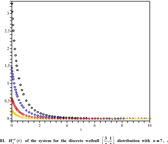
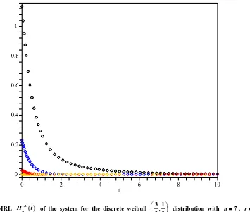
t is given by (8). Figures 1 and 2 show the graphs of

( )

,

r k n

H t in example 2.7

when 3

2

α= , 1

2

β = , n=7 for different values of r and k.

Remark 2.8 Let us consider again the condition random variable , , : :

r k n

t k n r n

T =T −t T ≥t for which the

survival function is given by (2). The representation (2) shows that Tt1, ,k n is in fact the k, the order statistics

Figure 1. The MRL r,k

( )

n

H t of the system for the discrete weibull _ , _

 

3 1

2 2 distribution with n=7, k=5, and , , ,

2 3 4 5

[image:6.595.156.498.418.712.2]

Figure 2. The MRL Hnr,k

( )

t of the system for the discrete weibull ,

 

 

 

3 1

2 2 distribution with n=7, r=3, and , , ,

3 4 5 6

k= from the top respectively.

form of a distribution with survival function

(

)

( )

1

S t x

S t

+ +

. Hence using the result of David and Nagaraje [8],

one can write

(

1, ,

)

( )

1

(

_{( )}

)

1

1 1

1 .

j n

j n k k n

t

j n k

S t x

j n

P T x

n k j S t

− + +

= − +

 + + 

−

  

> = −  _{−  } _

   

∑

Hence

( )

( )

1 1

( )

1

1 1

n

j n k k

n j

j n k

j n

H t H t

n k j

− + −

= − +

−

  

= − _{  }

−

  

∑

and

( )

1

( )

( )

, 1 1

0 1

1

( 1) .

r n i

r k j n k

n i j

i j n k

j n

H t P t H t

n k j

− −

− + − = = − +

−

  

= − _{  }

−

  

∑

∑

(9)

This indicates the MRL Hnr k,

( )

t can be expressed in terms of simpler MRL

( )

1

j

H t which is in fact the

MRL of series systems.

The following theorem gives bounds for Hnr k,

( )

t .

Theorem 2.9 It is always true that

( )

( )

( )

1 ,

1

k n r k k

n r n n

H − +− + t ≤H t ≤H t

Proof: The proof is similar to the proof of Theorem 2.3 of [4] and hence is omitted.

The next theorem proves that when the parent distribution has increased hazard rate, Hnr k,

( )

t increases in

[image:7.595.150.505.83.384.2]

Theorem 2.10 If h t

( )

is increasing in t, then Hnr k,

( )

t is decreasing in t .

Proof: In order to prove the result, we need to show that, for ,r k and n fixed,

( )

(

)

, ,

1 0.

r k r k

n n

H t −H t+ ≥

We have, from (8), after some algebra

( )

(

)

( )

( )

(

)

(

)

( )

(

( )

(

)

)

(

) ( )

(

(

)

)

1 1 , , 0 0 1 1 0 0

1 1 1

1 1 1

r r

r k r k k i k i

n n i n i i n

i i

r r

k i k i k i

i n i n i n i i i

i i

H t H t P t H t P t H t

P t H t H t H t P t P t

− − − − − = = − − − − − − − − = = − + = − + + = − + + + − +

∑

∑

∑

∑

But the first term in the above equality is positive by Theorem 2.2. Hence we just need to prove that the

second term in the above equality is positive. Assume that

( )

( )

( )

1 S t t

S t φ

−

= and note that φ

( )

t is an increasing function of t. Then

(

)

( )

( )

(

)

(

)

( ) (

)

(

(

)

(

)

)

( )

(

)

1 1 1 0 0

1 1 1 1

0

0 0 0 0

1 1 1 1

1

1 1

r r

i i i j k i k j

n i n j r

i j k i

n i _{r r}

r r

i j j j j

j j j j

n n n n

t t t t H t H t

j i j i

H t

n n n n

t t t t

j j j j

φ φ φ φ

φ φ φ φ

− − − − − − − _{= =} − − _{− − − −} = = = = =          + + + − +                   + _ − _=     ₊                   +  _{   }         

∑∑

∑

∑

∑

∑

∑

.    

After some algebraic manipulations, one can show that the numerator of the expression is equal to

(

)

( ) (

)

(

)

(

(

)

(

)

)

2 1

0 1

( ) 1 1 1 1 .

r r

i j j i k i k j n i n j i j i

n n

t t t t H t H t

i j φ φ φ φ

− − − − − − = = +    + − + + − +      

∑ ∑

(10)

It can be easily shown that for j>i, k i

(

1

)

k j

(

1 > 0

)

n i n j

H ₋− t+ −H ₋− t+ (see, [2,3]). On the other hand, as φ

( )

t

is an increasing function of t, we have

(

φi

( ) (

t φj t+ −1

)

φj

( ) (

t φi t+1

)

)

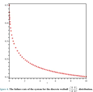
≥0. This implies that the expression in (10) is non-negative and hence the proof is complete.

Remark 2.11 As it was already mentioned for a system with decreasing failure rate components, Hnk

( )

t is

increasing in time. This result, however, is not generally true for MRL Hnr k,

( )

t . Figures 3 and 4 show the

graphs of h t

( )

and Hnr k,

( )

t in Example 2.7. As the graphs show that h t

( )

is a decreasing function of time,

however, Hnr k,

( )

t is an increasing function of t for a period of time and then starts to decrease.

Remark 2.12 In the following, we show that P t_i

( )

has its own interesting interpretation. In fact, under the condition that the system is working at time t, P t_i

( )

shows the probability that there is exactly i com- ponent failure in the system. The mentioned conditional probability can be written as

(

) (

) (

)

(

)

(

)

(

(

)

)

( )

(

)

( )

( )

(

)

( )

( )

(

)

( )

( )

(

)

( )

: 1: : : : 1: :

: : 1: :

: : 1 1 1 1 1 0 0 1 1 1 1

i n i n r n i n r n i n r n i n r n i n r n

r n r n

r r

j _{n j} j _{n j}

j i j i

r _j r _j

n j n j

j j

P T t T T t P T t T t P T t T t

P T t T P T t T

P T t P T t

n n

S t S t S t S t

j j

n n

S t S t S t S t

j j n j + + + − − − − = = + − − − − = =

< < ≥ = < ≥ − < ≥

< ≤ < ≤

= − ≥ ≥     − −         = −     − −          =

∑

∑

∑

∑

( )

(

)

( )

( )

(

)

( )

( )

( )

( )

1 1 0 0 1 1

, 0, , 1

i _{n i i}

r _j r

n j j

j j

i

n

S t S t t

j

n n

S t S t t

j j

P t i r

[image:9.595.168.456.86.383.2]

Figure 3. The MRL r,k

( )

n

H t of the system for the discrete weibull _ , _

 

1 1

2 2 distribution with n=7, k=5, and 5

[image:9.595.155.476.412.732.2]

r= .

Figure 4. The failure rate of the system for the discrete weibull _ , _

 

1 1

where

( )

( )

( )

1 S t t

S t

φ = − for t such that S t

( )

> 0 shows the odds of the event that a component has a lifetime

less than t. Also in the following, we study some properties of P ti

( )

.

Theorem 2.13 For i=0 P t_i

( )

is decreasing function of t and for i= −r 1, it is increasing function of t. Also, for 0≤ ≤ −i r 1

( )

0

1 0

lim

0 0

i t

i P t

i

→

= 

=  _≠



( )

1 1

lim

0 1

i t

i r

P t

i r

→∞

= − 

=  _{≠ −}



Proof: We have

( )

( )

0 ₁

=0

1

r j j

P t

n t

j φ

−

=      

∑

(11)

which is obviously a decreasing function of t (φ

( )

t is a increasing function) since limt→0φ

( )

t =0 and

( )

1

limt→∞φ t = . From (11), we easily conclude that limt→0 0P t

( )

=1 and limt→∞P t0

( )

=0.

( )

( )

1 ₁

1

0

1 .

r _r

j r j

n r

P t

n

t

j φ

− ₋

− + =

 

 ₋ 

 

=      

∑

In this case, it is easily seen that Pr−1

( )

t is an increasing function of t , limt→0Pr−1

( )

t =0 and

( )

1 1

limt→∞Pr− t = .

Theorem 2.14 The survival function S t

( )

can be uniquely determined by P ti

( )

and Pi+1

( )

t ,

0,1, , 1

i=  r− as follows:

( )

₍

_{) ( ) (}

(

) ( )

₎

_{( )}

1 . 1

i

i i

n i P t S t

n i P t i P₊ t

− =

− + + (12)

Proof:

The result easily follows from the fact that for i=0,,r−1,

( )

( )

( )

( )

1 1

, 1

i i

P t n i S t

P t i S t

+ ₌ − _⋅ −

+

which gives (12).

Consider the vector P

( )

t =

(

P t0

( )

,,Pr−1

( )

t

)

. Obviously, P

( )

t is a probability vector. we can then prove

the following theorem.

Theorem 2.15 For all 0≤ ≤t1 t2,

( )

t1 ≤_st

( )

t2 .

P P

Proof: In order to prove the result, we need to show that for j=0,,r−1,

( )

( )

1 1

1 2 , 0, , 1

r r

i i

i j i j

P t P t j r

− −

= =

≤ = −

∑

∑



( )

( )

( )

( )

1 1

1 2

1 1

1 2

0 0

.

r r

i i

i j i j

r r

k k

k k

n n

t t

i i

n n

t t

k k

φ φ

φ φ

− −

= =

− −

= =

   

   

  _≤  

   

   

   

∑

∑

∑

∑

This is equivalent to show that

( )

( )

( )

( )

1 1

2 1

0 0

1 1

2 1

j j

k k

k k

r r

i i

i j i j

n n

t t

k k

n n

t t

i i

φ φ

φ φ

− −

= =

− −

= =

   

   

  _≤  

   

   

   

∑

∑

∑

∑

or

( ) ( )

( ) ( )

(

)

1 1

2 1 1 2

0

0.

j r

k l k l k l j

n n

t t t t

k l φ φ φ φ

− −

= =

   _{− ≤}

     

∑∑

(13)

But, as φ

( )

t is increasing in t, the bracket in the summations, for k<l, is always negative. Hence the inequality in (13) is valid. This completes the proof of the theorem.

Theorem 2.16 Consider two

(

n− +k 1

)

-out-of-n systems. Assume that the components of the systems have independent lifetimes, with survival function S t1

( )

and S2

( )

t , respectively and odds functions φ1

( )

t and

( )

2 t

φ , respectively. If for all t, S t1

( )

≤S2

( )

t , then P1

( )

t ≥_st P2

( )

t .

Proof: Asadi & Berred [16] proved that

( )

1

,

1 0

r k k i i

r n

r i j

n t k t

n t j η

− =

− =

      =

     

∑

∑

for fixed

i and n is an increasing function

of t.

The assumption that S t1

( )

≤S2

( )

t implies φ1

( )

t ≥φ2

( )

t , then

( )

(

)

(

( )

)

, 1 , 2

i i

r n t r n t

η φ ≥η φ

which is equivalent to say that for all i=0,,r−1 and all t,

( )

( )

( )

(

( )

( )

)

1 1

1 2

01 02

1 1

1 2

0 0

( )

, .

r r

k k

k i k i

st

r r

j j

j j

n n

t t

k k

P t P t

n n

t t

j j

φ φ

φ φ

− −

= =

− −

= =

   

   

  _≥   _≥

   

   

   

∑

∑

∑

∑

REFERENCES

[1] I. Bairamov, M. Ahsanullah and I. Akhundov, “A Residual Life Function of a System Having Parallel and Series Structures,”

Journal of Statistical Theory and Applications, Vol. 1, No. 2,2002, pp. 119-132.

[2] M. Asadi and I. Bairamoglu, “A Note on the Mean Residual Life Function of the Parallel Systems,” Communications in Statis-tics Theoy and Methods, Vol. 34, No. 2, 2005, pp. 1-12.

[3] M. Asadi and I. Bairamoglu, “On the Mean Residual Life Function of the k-out-of-n Systems at System Level,” IEEE Transac-tions on Reliability, Vol. 55, No. 2,2006, pp. 314-318. http://dx.doi.org/10.1109/TR.2006.874934

[4] M. Asadi and S. Goliforushani, “On the Mean Residual Life Function of Coherent Systems,” IEEE Transactions on Reliability, Vol. 57, No. 4,2008, pp. 574-580. http://dx.doi.org/10.1109/TR.2008.2007161

[5] X. Li and P. Zhao, “Stochastic Comparison on General Inactivity Time and General Residual Life of k-out-of-n Systems,”

Communications in Statistics—Simulation and Computation, Vol. 37, No. 5,2008, pp. 1005-1019. http://dx.doi.org/10.1080/03610910801943784

[7] X. Li and Z. Zhang, “Some Stochastic Comparisons of Conditional Coherent Systems,” Applied Stochastic Models in Business and Industry, Vol. 24, No. 6,2008, pp. 541-549. http://dx.doi.org/10.1002/asmb.715

[8] J. Navarro, N. Balakrishnan and F. J. Samaniego, “Mixture Reptesentations of Residual Lifetimes of Used Systems,” Journal of Applied Probability, Vol. 45, No. 4, 2008, pp. 1097-1112. http://dx.doi.org/10.1239/jap/1231340236

[9] Z. Zhang, “Ordering Conditional General Coherent Systems with Exchaneable Components,” Journal of Statistical Planning and Inference, Vol. 140, No. 2,2010, pp. 454-460. http://dx.doi.org/10.1016/j.jspi.2009.07.029

[10] Z. Zhang, “Mixture Representations of Inactivity Times of Conditional Coherent Systems and Their Applications,” Journal of Applied Probability, Vol. 47, No. 3,2010, pp. 876-885. http://dx.doi.org/10.1239/jap/1285335415

[11] Z. Zhang and X. Li, “Some New Results on Stochastic Orders and Aging Properties of Coherent Systems,” IEEE Transactions on Reliability, Vol. 59, No. 4,2010, pp. 718-724. http://dx.doi.org/10.1109/TR.2010.2087431

[12] M. Kelkin Nama and M. Asadi, “Stochastic Properties of Components in a Used Coherent Systems,” Methodology and Compu-ting in Applied Probability, 2013.http://dx.doi.org/10.1007/s11009-013-9322-2

[13] J. Mi, “Limit of Hazard Rate Function of Coherent System with Discrete Life,” Applied Stochastic Models in Business and Industry, Vol. 27, No. 5,2010, pp. 711-717.

[14] H. A. David and H. N. Nagaraja, “Order Statistics,” 3rd Edition, John Wiely & Sons, New York, 2003. http://dx.doi.org/10.1002/0471722162

[15] M. Khorashadizadeh, A. H. Rezaei Roknabadi and G. R. Mohtashami Borzadaran, “Variance Residual Life Function in Dis-crete Random Ageing,” Metron, Vol. 1, No. 1,2010, pp. 57-67.