The Effect of Pseudo exogenous Instrumental Variables on Hausman Test

Munich Personal RePEc Archive

The Effect of Pseudo-exogenous

Instrumental Variables on Hausman Test

Jeong, Jinook and Yoon, Byung

Yonsei University

April 2007

Online at

https://mpra.ub.uni-muenchen.de/9792/

The Effect of Pseudo-exogenous Instrumental Variables on

Hausman Test

by

Jinook Jeong1 School of Economics

Yonsei University

and

Byung Ho Yoon School of Economics

Yonsei University

April 2007

Abstract

This paper investigates the potential problem of ‘pseudo-exogenous’ instruments in regression models. We show that the performance of Hausman test is deteriorated when the instruments are asymptotically exogenous but endogenous in finite samples, through Monte Carlo simulations.

Keywords: Hausman test, endogeneity, instrumental variable

JEL classifications: C12, C15

Acknowledgement: We are grateful for the helpful comments from Professor Dong H. Kim and the participants of NAIS conference at Yonsei University. This research has been financially supported by Suam Foundation. The authors are members of ‘Brain Korea 21’ Research Group of Yonsei University.

1 _{Corresponding Author, 1) address: School of Economics, Yonsei University, Seoul,}

I. Introduction

When there exist endogenous explanatory variables in a regression model, the least

squares estimator fails to achieve consistency. To identify the endogeneity of the

explanatory variables, Hausman test is widely employed. Hausman test works pretty

well, but it is not free of problems. Meepagala (1992) shows that the power of Hausman

test decreases as the sample size becomes smaller. Staiger and Stock (1994) show that

‘weak’ instruments weaken the power of Hausman test. Wong (1996) proposes a

bootstrap procedure to improve the finite sample properties of Hausman test when the

instruments are weak.

This paper identifies another potential problem of Hausman test. When the

instruments of IV estimation are correlated with the error term of the regression, although

the correlation converges to zero eventually, the finite sample performance of Hausman

test becomes seriously deteriorated. Let us call such instruments, which are

asymptotically exogenous but endogenous in the finite sample, ‘pseudo-exogenous’

instruments. Pseudo-exogenous instruments, of course, do not affect the asymptotic

distribution of Hausman test. However, as we will show through a series of Monte Carlo

experiments, the empirical sizes and powers of Hausman test could be considerably

inaccurate in finite samples. Especially, we will show the empirical power function of

Hausman test actually ‘collapses’ in some cases.

One of the most popularly used instruments is the fitted value of the endogenous

variable from the reduced form regression. This so-called 2SLS (two-stage least

squares) is widely used as it gives a proper instrument. Such a fitted value is by

construction a pseudo-exogenous instrument. The correlation between the fitted value

II. Hausman Test with the Pseudo-exogenous Instrument

Let us consider the following model.

u x y= β+

where is an ( ×1) vector of explanatory variable, is an ( ×1) vector of error

terms, and is an ( ×1) vector of dependent variable. Suppose there exists an ( ×1)

vector of the instrumental variable, z . We are interested in testing : “x is

exogenous” against : “x is endogenous.” By a similar derivation as in Bound et al.

(1995), it is straightforward that

x N u N

y N 1 H N 0 H 2 x xu 1

ols plim(x'x) x'y

ˆ im pl σ σ + β = = β − xz zu 1

iv plim(z'x) z'y ˆ im pl σ σ + β = = β −

where )

N u ' x ( m pli xu ≡

σ , )

N u ' z ( m pli zu ≡

σ , )

N z ' x ( m pli xz ≡

σ and )

N x ' x ( m pli 2 x ≡ σ .

First, suppose that z is exogenous so that 0 xz zu = σ σ

. Let us define

. If is exogenous (i.e. is true) as well as , then

) ˆ ˆ ( m pli

q≡ β_iv −β_ols x H₀ z

0 xz zu 2 x xu = σ σ = σ σ

and q=0. If is still exogenous but is endogenous (i.e. is

true), then

z x H₁

0 xz zu = σ σ

and ₂

x xu

σ σ

q= − . Now Hausman statistic H is

[

]

) ˆ ˆ (

H≡ β_iv−β_ols ′ β_iv − β_ols −1 β_iv−β_ols

which converges to zero under and diverges from zero under . It has been

shown by Hausman (1978) that Hausman statistic has an asymptotic distribution

is not exogenous at all. In this case, Hausman test is not

define

0

H , H₁

χ2

under H . ₀

Second, suppose z

d well. If z is not exogenous, then 0 xz zu ≠ σ σ

. Thus, even when x is

exogenous (i.e. H₀ is true), q is not zero any longer but xz zu σ σ

endogenous (i.e. H₁ is true), q is now zu xu₂ σ_x xz σ − σ σ

. Thus, Haus statistic H no

longer converges t zero under H , and is no longer guaranteed to diverge from ero ₀

1

are as totically exogenous but endogenous the finite sample. In th c man

under . , the null distribution of is no longer an asymptotic

Third, let us consider the case of ‘pse instrumental variables, which

se,

Hausm

is e the

z

2 .

s a o

Accordingly

III. Monte Carlo Simulation

d. Consider

H ymp utio perform H udo-exogenous’ in er

ng data generating process (DGP):

χ

i

an test is well-defined in large samples, but could be problematic in small samples.

Although q≡plim(βˆ_iv −βˆ_ols)=0under H and ₀ q≡plim(βˆ_iv −βˆ_ols)≠0 under H₁, as

0 ) u ' z (

E ≠ in finite samples, the Hausman statistic, H , may not be close enough to zero

under H₀ enoug rom z finite sample

of Hausman statistic may not be χ2 eith The following section examines

the effect of the pseudo-exogenous instrument on Hausman test through simulations.

To substantiate the effect of the pseudo-exogenous instrument, a Monte Carlo study and/or distinguishe

n

d

followi

h f o under H₁ . The

er. distrib

u x

y= β+

where ⎟ ⎟ ⎟ ⎠ ⎞ ⎜ ⎜ ⎜ ⎝ ⎛ ⎥ ⎥ ⎥ ⎦ ⎤ ⎢ ⎢ ⎣ ⎡ ⎥ ⎥ ⎥ ⎦ ⎤ 2 u s a

⎢ , ρ ρ ρ ρ ρ ρ ⎢ ⎢ ⎢ ⎣ ⎡ = ⎟⎟ ⎟ ⎟ ⎠ ⎥ ⎥ ⎥ ⎦ ⎤ ⎢ ⎢ ⎢ ⎣ ⎡ ⎟ ⎟ ⎟ ⎠ ⎞ 1 N 20 N 20 1 1 0 0 0 N s s s s s , N ~ zu xu zu xz xu xz 2 u xu zu xz xu x i i i

where i = 1, 2, …, N For sim , nd ⎞ 2 ⎜⎜ ⎜ ⎜ ⎝ ⎛ ⎥ ⎥ ⎥ ⎦ ⎤ ⎢ ⎢ ⎢ ⎣ ⎡ 0 0 0 . ⎜ ⎜ ⎜ ⎝ ⎛ u z x s s s licity s zu 2 z xz

p s , 2_x s , 2_z β are all set to one. ake

the instrument ‘pseudo-exogenous,’ is defined as

To m zu s N 20 s zu zu ρ

≡ . Note that the

l 2

in finite samples. As the sam le size zu, ρ

p

correlation coefficient between z and u in a sampe size of 0 (N=20), is not set to always

increases, however, s converses to zero (i.e. the instrument becomes exogenous). _zu

Thus, z is a ‘pseudo-exogenous’ instrument. The correlation coefficient between x and z,

xz

ρ is set to 0.7 so that we can avoid the so-called ‘weak instrument’ problems. Four

alternative sample sizes are considered: 20, 50, 100, and 500 for comparisons. The

ulation has been performed 1,000 times.

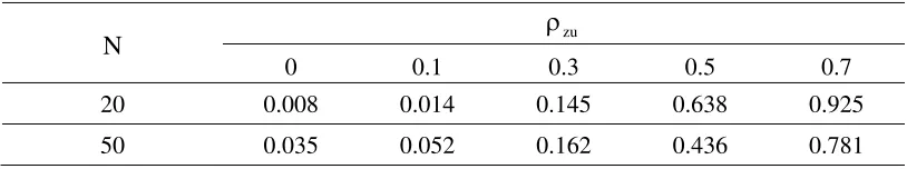
Table 1 and Figure 1 present the empirical sizes of Hausman test. First, we notice

that the empirical size of Hausman test is not accurate in small samples even when the

u sim

instr ment is perfectly exogenous (ρ_zu=0). For instance, when N=20 and ρ_zu=0, the

rejection rate is only 0.008 while the nominal size is 0.05. Second, when the instrument

is pseudo-exogenous (i.e. ρ_zu≠0), mpirical sizes of Hausman test are seriously

distorted. For example, when N=20 and _zu 0.7 the e

=

ρ , Hausman test rejects the true null

empirical size is far from accurate even whe : the empirical size is 13.6% while

the nominal size is 5%.

hypothesis 925 times out of 1,000 simulations: the empirical size is 92.5% while the

inal size is 5%. ch size distortion fades away as the sample size grows, but the

n N=500

ble 1 Empirical sizes of Hausman test (

nom Su

Ta 2

% 5

=

α )

N ρzu

0 0.1 0.3 0.5 0.7

20 0.008 0.014 0.145 0.638 0.925

50 0.035 0.052 0.162 0.436 0.781

2 _{We experimented how big the sample size (N) should be to achieve an accurate}

100 0.035 0.047 0.108 0.269 0.467

500 0.058 0.047 0.066 0.095 0.136

Figure 1 Empirical sizes of Hausman test (α =5%)

Actual Sizes of Haus st

0 0.2 0.4 0.6 0.8 1

0 0.1 0.2 0.3 0.4 0.5 0.6 0.7

Cor(z,u)

Actu

al sizes

man Te

N=20 N=50 N=100 N=500

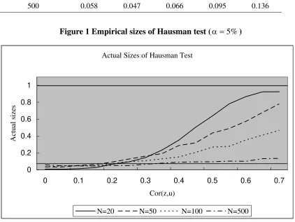
Table 2 shows the empirical powers of Hausman test. First of all, it is obvious

that Hausman test does not work well in small samples when the instrument is

pseudo-exogenous. For example, even when ρ_xu=0.7, Hausman test does not easily reject the

false null hypothesis H0: 0ρ_xu = in N = 20 cases, if ρ_zu ≠0: the empirical powers are

7.6% (for ρ_zu =0.3), 1.4% (for ρ_zu =0.5), and 12.3% (for ρ_zu =0.7). Generally, the

empirical po 0 s showing higher

a p owers become a

case (

wers are ex

powers than 10% in T

1 . 0

= and

exogeneity of the instrum trem

ble 2. Wh

7 . 0 =

ent

ely low when N = 2 , only a few exception

le size is 50, the em

ite a fe

). It should be noted that even when the

pseudo-1 . 0 en the sam

is quite weak (such as

pirical p

bit higher, but still show powers lower than 10% in qu w cases. Even when the

sample size is 100, Hausman test rejects only 13.7% of the false null hypothesis in some

xu zu

zu

ρ ρ

=

ρ ), the empirical power of

Hausman test could be pretty low in small samples. For example, in the case of ρ_xu=

ma

decreases to 0.120 for ρ_zu=0.1. It implies that, in small samples, Hausman test could be

distorte eak co between the instrument and the error term even though

Table 2 Empirical power of Hausman test ( 5%

d by a w ation

they are asymptotically independent. rrel

=

α )

xu

ρ N ρzu

0 0.1 0.3 0.5 0.7

0.1

20 0.010 0.008 0.079 0.468 0.890

50 0.070 0.038 0.058 0.157 0.465

100 0.149 0.088 0.039 0.042 0.137

500 0.607 0.527 0.473 0.331 0.272

0.3

008 0.008 0.140 0.712 20 0.054 0.

50 0.493 0.316 0.100 0.035 0.068

100 0.859 0.787 0.547 0.329 0.151

500 1.000 1.000 1.000 1.000 0.999

0.5

20 0.342 0.120 0.011 0.031 0.383

50 0.986 0.953 0.697 0.296 0.070

100 1.000 1.000 0.999 0.990 0.934

500 1.000 1.000 1.000 1.000 1.000

0.7

20 0.900 0.746 0.076 0.014 0.123 50 1.000 1.000 1.000 0.981 0.774 100 1.000 1.000 1.000 1.000 1.000 500 1.000 1.000 1.000 1.000 1.000

Second, the empirical powers of Hausman te

increases ntuit pow xpected to become as th nitude of

the instrument ndog =

st show quite irregular variations as

zu

ρ . I iv

en

ely, the er is e lower e mag

’s e eity ( ρ_zu) becomes As shown in Ta ,

intuition. Som the power becomes

as com (f le, see se of

higher. ble 2, however

the em

higher

pirical powers do not support such

es

etimes

be higher or examp the ca ρ_xu=0 zu

ρ .3 and , among

oth while etimes the power becomes lo s expected. It is apparent from

Ta co cy at The reason why the

N=20

ers), som wer a

empir

con

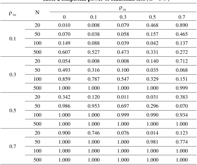
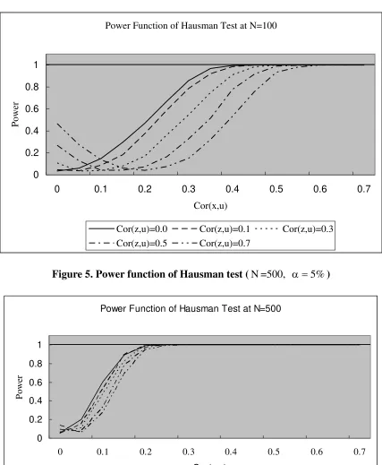
The empirical power functions depicted in Figures 2-5 confirm

Figure 2 presents the empirical power function of Hausman test when N = 20 for various

0 1

ical powers are inconsistent is explained in section II. Although (βˆ_iv−βˆ_ols)

verges to zero under H0 and to a positive number under H1 in large samples, it could

well be non-zero under H0 and zero under H1 in small samples. As a result, Hausman

statistic is not defined well.

values of ρ . Unlike a typical power function, they do not either approach to the

nominal size under H , nor approach to 1 under extreme H . When the magnitude of

pseudo-exogeneity is high (for example, _zu 0.7

such irregularities.

zu

=

ρ ), the power function goes even the

opposite way. As sample size grows, such an odd behavior weakens a little. However,

even when N = 50 and N = 100, the power function ‘collapses’ at around ρ_zu =0.35 and

15 . 0 zu =

Figure 2. Power function of Hausman test (N=20, α=5%)

Power Function of Hausman Test at N=20

0 0.2 0.4 0.6 0.8 1

0 0.1 0.2 0.3 0.4 0.5 0.6 0.7

Cor(x,u)

Po

w

er

Cor(z,u)=0.0 Cor(z,u)=0.1 Cor(z,u)=0.3

Cor(z,u)=0.5 Cor(z,u)=0.7

Figure 3. Power function of Hausman test (N=50, ρ_xz=0.7, α=5%)

Power Function of Hausman Test at N=50

0 0.2 0.4 0.6 0.8 1

0 0.1 0.2 0.3 0.4 0.5 0.6 0.7

Cor(x,u)

Po

w

er

Cor(z,u)=0.0 Cor(z,u)=0.1 Cor(z,u)=0.3

Figure 4. Power function of Hausman test (N=100, α=5%)

Power Function of Hausman Test at N=100

0 0.2 0.4 0.6 0.8 1

0 0.1 0.2 0.3 0.4 0.5 0.6 0.7

Cor(x,u)

Power

Cor(z,u)=0.0 Cor(z,u)=0.1 Cor(z,u)=0.3 Cor(z,u)=0.5 Cor(z,u)=0.7

Figure 5. Power function of Hausman test (N=500, α=5%)

Power Function of Hausman Test at N=500

0 0.2 0.4 0.6 0.8 1

0 0.1 0.2 0.3 0.4 0.5 0.6 0.7

Cor(x,u)

Po

w

er

Cor(z,u)=0.0 Cor(z,u)=0.1 Cor(z,u)=0.3

IV. Conclusion

While the problems of ‘weak’ instruments in IV estimation have been thoroughly

studied 3, the problems that ‘endogenous’ instruments may create have not been studied to

a great extent. This paper examines the effects of ‘pseudo-exogenous’ instruments on

Hausman test in finite samples. We show that the size and power of Hausman test could

be very inaccurate in finite samples when the instruments are pseudo-exogenous.

Researchers need to be cautious about the exogeneity of the instruments when they use IV

estimation in practice.

References

Bound, J., D. A. Jaeger and R. M. Baker (1995) “Problems with Instrumental Variables Estimation When the Correlation Between the Instruments and the Endogenous Explanatory Variable is Weak,” Journal of the American Statistical Association 90 (430), 443-450.

Hausman, J. A. (1978) “Specification Tests in Econometrics,” Econometrica 46(6), 1251-1270.

Maddala, G.S. and J. Jeong (1992), “On the Exact Small Sample Distribution of the Instrumental Variable Estimator,” Econometrica 60, pp.181-183.

Meepagala, G.. (1992) “On the Finite Sample Performance of Exogeneity Tests of Revankar, Revankar and Hartley and Wu-Hausman,” Econometric Review 11, 337-353.

Wong, K. (1996) “Bootstrapping Hausman’s exogeneity test,” Economics Letters 53(2), 139-143.