Munich Personal RePEc Archive
Calculating the Fundamental Equilibrium
Exchange Rate of the Macedonian Denar
Jovanovic, Branimir
Staffordshire University, UK
2007
Online at
https://mpra.ub.uni-muenchen.de/43161/
CALCULATING THE FUNDAMENTAL EQUILIBRIUM
EXCHANGE RATE OF THE MACEDONIAN DENAR
JOVANOVIK, Branimir
This dissertation is submitted in partial fulfilment of the requirements of
Staffordshire University for the award of MSc Economics for Business Analysis
EXECUTIVE SUMMARY
The real exchange rate is a macroeconomic variable of a crucial importance, since it
determines relative price of goods and services home and abroad, and influences economic
agents’ decisions. The real exchange rate needs to be on the right level, as it can result in
wrong signals and economic distortions if it is not. In order to be able to say whether a
currency is misaligned or not, one needs some measure of the just exchange rate – the
equilibrium exchange rate.
Many different concepts of equilibrium exchange rates exist. The one which is defined as the
real effective exchange rate that is consistent with the economy being in internal and external
equilibrium in the medium term is the subject of this thesis, and is known under the name of
Fundamental Equilibrium Exchange Rate concept. The first part of this study, thus, explains
the concept of Fundamental Equilibrium Exchange Rate and surveys the literature on the
uses to which it has been put and on the ways in which it has been calculated. The second
part of the dissertation illustrates how the Fundamental Equilibrium Exchange Rate concept
can be operationalised towards the end of assessing the right parity of the Macedonian
denar.
What we find is that the denar is neither overvalued nor overvalued in the period 1998-2005.
That would imply that price competitiveness is not adversely affected, and that the exchange
rate does not generate distortions in the economy. We also find that the fundamental
equilibrium exchange rate tends to appreciate due to the increase in the net current transfers
flows. In contrast, the real effective exchange rate tends to depreciate in the last three
periods, and we are of the opinion that if these trends are maintained, in near future the
ACKNOWLEDGEMENTS
This dissertation would never come to existence if the Foreign and Commonwealth Office,
the Open Society Institute and the Staffordshire University did not grant me the opportunity
to study at this programme. Since they did, I would like to express my gratitude to Prof.
Geoff Pugh for his invaluably useful comments and critical suggestions, to Prof. Jean
Mangan, for her comments and willingness to help, and to Igor Velickovski and Sultanija
Bojceva-Terzijan for their help with the data.
LIST OF CONTENTS
CHAPTER 1: Introduction
CHAPTER 2: Literature Review on FEER
Introduction
2.1. Exchange rate misalignment 2.2. Purchasing Power Parity 2.3. How is FEER defined? 2.4. Understanding the FEER 2.5. Further discussion 2.6. How is FEER estimated?
CHAPTER 3: Estimating the FEER of the denar
Introduction 3.1. Methodology 3.2. Data
3.3. Discussion about the characteristics of the Macedonian economy 3.4. Tests of order of integration of the series
3.5. Estimating the trade equations ARDL estimates
Johansen estimates
3.6. Obtaining the equilibrium values 3.7. Selecting the current account target 3.8. Sensitivity analysis, discussion and results 3.9. Potential drawbacks
CHAPTER 4: Main findings, conclusions and recommendations for further research References
1 3
3 3 5 7 8 10 12
19
19 19 21 24 29 31 31 42 48 53 55 62
LIST OF FIGURES, TABLES AND APPENDICES
Figure 1 Figure 2 Figure 3 Figure 4 Figure 5 Figure 6 Figure 7 Figure 8 Figure 9 Figure 10 Figure 11 Figure 12 Figure 13 Figure 14 Figure 15 Figure 16 Figure 17 Figure 18 Figure 19 Figure 20 Figure 21 Figure 22 Figure 23 Figure 24 Figure 25 Figure 26 Figure 27 Figure 28 Figure 29 Figure 30 Table 1 Table 2 Table 3 Table 4 Table 5 Table 6 Table 7 Table 8 Table 9 Table 10 Table 11 Table 12 Table 13 Table 14 Table 15 Table 16 Table 17 Table 18 Table 19 Table 20 Appendix 1 Appendix 2 Appendix 3 Appendix 4FEER, the exchange rate consistent with internal and external balance Macedonian import volumes, 1998-2005
Macedonian export volumes, 1998-2005 Macedonian export prices, 1998-2005 Macedonian GDP, 1998-2005 Foreign demand, 1998-2005
Real Effective Exchange Rate of the denar
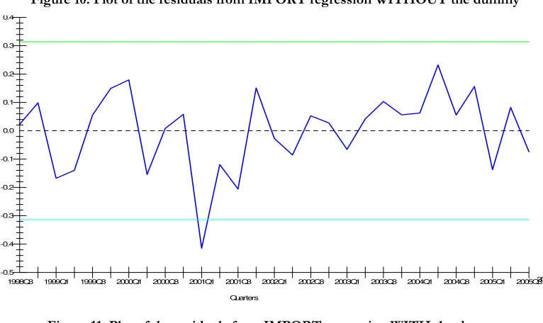
Plot of the residuals from EXPORT regression WITHOUT the dummy Plot of the residuals from EXPORT regression WITH the dummy Plot of the residuals from IMPORT regression WITHOUT the dummy Plot of the residuals from IMPORT regression WITH the dummy Plot of the residuals from EXPORT regression WITHOUT dummies Plot of the residuals from EXPORT regression WITH dummies Plot of the residuals from IMPORT regression WITHOUT the dummy Plot of the residuals from IMPORT regression WITH the dummy Macedonian GDP, original and filtered
Foreign demand, original and filtered Export prices, original and filtered Import prices, original and filtered Interest flows, original and filtered Net transfers, original and filtered Current account targets
REER and FEER1
REER, FEER1 and FEER2
FEER1, FEER3, FEER4, FEER5 and FEER6 FEER1, FEER7, FEER8
Net transfers, % of GDP FEER1 and FEER9
FEER1, FEER10 and FEER11 Different FEERs
Structure of Macedonian exports by countries
Trade balance, net transfers and current account, as % of GDP Unemployment and inflation rates
Results of the test of the hypothesis that the series are non-stationary Results of the tests for unit root in the first differences series Criteria for choosing the number of lags in the ARDL Regressions with and without dummy
Results of the test of a long-run relationship
Results of the test of long-run relationship with changed dependent variable Long run coefficients and probability values for EXPORT regression Long run coefficients and probability values for IMPORT regression Diagnostics for different orders of the VAR for EXPORTS
Diagnostics for different orders of the VAR for IMPORTS
The Schwarz Bayesian Criterion and the Akaike Information Criterion Tests for the number of cointegrating vectors
The cointegrating vectors
Comparison between the coefficients obtained by the two methods Test whether the Johansen EXPORT elasticities differ from the ARDL Test whether the Johansen IMPORT elasticities differ from the ARDL Different FEERs
Data
Unit root tests
ARDL estimates of the trade equations Johansen estimates of the trade equations
CHAPTER 1 Introduction
The real exchange rate is well recognised in the economic literature as one of the key
macroeconomic variables. Being defined as the relative price of a common basket of goods
domestically and internationally measured in the same numeraire (i.e. price-adjusted nominal
exchange rate), it determines price competitiveness and affects the consumption and
production decisions of the economic agents, and hence trade, economic activity,
unemployment and inflation.
The variability of the exchange rate, as well as the consequences of it, has not been
overlooked in the economic literature either. Two dimensions of variability can be identified:
exchange rate volatility is the change of the rate from one point of time to another; exchange rate misalignment is the departure of the exchange rate from its equilibrium value (Williamson 1983). While the costs associated with volatility have attracted significant attention1, leading
often to variability being identified with volatility, the costs associated with misalignments
have often been overlooked. However, as Williamson (1983, p. 45) states, while exchange
rate volatility is a troublesome nuisance, exchange rate misalignment is a major source of
concern, generating ‘austerity, adjustments costs, recession, deindustrialization, inflation and
protectionism’. In addition, as Stein and Paladino (1999) argue, misalignments may lead to
speculative attacks.
The identification of misalignments, thus, requires identification of the equilibrium level of
the exchange rate. Several methods for this purpose exist2, with one of the most popular and
most widely used being the Fundamental Equilibrium Exchange Rate concept. This
dissertation will engage with both the theoretical foundations of this concept and its
application to the Macedonian denar. There has been a substantial academic debate lately
with respect to the exchange rate of the Macedonian denar, with a prevailing opinion that
the denar is overvalued, and that this affects adversely the performances of the Macedonian
economy. However, while the debate in the academic circles is sound and ongoing, it has
been characterised with a lack of researches on the issue. This dissertation will therefore
illustrate how the Fundamental Equilibrium Exchange Rate concept can be applied to assess
whether the Macedonian denar is overvalued or undervalued.
The dissertation is organised as follows: in Chapter 2 the theoretical issues regarding the
Fundamental Equilibrium Exchange Rate are discussed. After the costs of misalignment are
presented and the most popular method for estimating the equilibrium exchange rate, the
Purchasing Power Parity method is assessed, the definition of the Fundamental Equilibrium
Exchange Rate and its distinctive characteristic – its medium-term nature – are discussed.
The final section of Chapter 2 surveys the different approaches in the literature to calculating
the Fundamental Equilibrium Exchange Rate. In Chapter 3 one of these approaches, the
partial equilibrium approach, is operationalised for calculating the Fundamental Equilibrium
Exchange Rate of the denar. As the Fundamental Equilibrium Exchange Rate estimates are
believed to be extremely sensitive on the underlying assumptions, great attention is paid to
this issue. Additionally, an analysis of the sensitivity of the calculations with respect to
different assumptions is carried out, and a range of alternative estimates is presented. The
findings turn out to be robust to the assumptions, and the reasons explaining the findings
are then discussed. Chapter 3 concludes with a discussion on the possible weaknesses of the
research, arguing that most of them are of an objective nature and arise from data
limitations. In Chapter 4 the conclusions we find are presented, and recommendations for
CHAPTER 2
Literature Review on FEER
‘The concept of the equilibrium exchange rate is an elusive one.’
Williamson (1994, p. 179)
In this chapter the theoretical foundations of the Fundamental Equilibrium Exchange Rate
(FEER) concept are explained. As an introduction to the discussion, the costs of exchange
rate misalignment are pointed out. Then the most popular concept for assessing whether a
currency is misaligned or not, the Purchasing Power Parity is explained and critically
evaluated. The discussion on the FEER begins with a survey on the development of the
concept and its use. Then the definition of the FEER is explained in more depth, and the
distinctive characteristic of the concept, its medium-term nature, is analyzed. Issues related
to the calculation of the fundamental equilibrium exchange rate are considered in the final
section, when the most important studies on FEER calculation are briefly explained.
2.1. Exchange rate misalignment
Real exchange rate as a macroeconomic variable determines the relative price of domestic
products relative to foreign, and therefore directly influences exports and imports and thus
aggregate demand, output, unemployment and inflation. Real appreciation decreases price
competitiveness, lowers the demand for domestic products, decreases exports and increases
imports, inhibiting economic activity, raising unemployment and lowering inflation; the
opposite happens with real depreciation.
‘The impact of exchange rate misalignment … on economic development has been, and
continues to be, deleterious’ (Yotopoulos and Sawada 2005, p. 10). Therefore, it is surprising
that the costs associated with a misaligned exchange rate, i.e. the departure of the exchange
rate from its equilibrium level, have received so little attention in the economic literature
The costs of exchange rate misalignment are mainly seen as higher unemployment when the
currency is overvalued and higher inflation when it is undervalued. However, as Williamson
(1983) argues, exchange rate misalignments incur other costs, as well. First, to maintain full
employment in presence of overvaluation, the decline in the demand for tradable goods will
have to be offset by an increased demand for non-tradable goods; this increases
consumption over the sustainable level and results in trade deficits. Sooner or later,
devaluation will have to occur to make up for the accumulated trade deficits, when the
consumption will have to be cut down, below the sustainable level. These variations in
consumption are costly, as people are made worse off, given that according to the
‘permanent income hypothesis’ they tend to even up their consumption. Second, there are
costs associated with the reallocation of the resources between tradable and non-tradable
industries, e.g. costs for retraining the workers and for adjustment of the capital equipment.
Third, some companies might be able to work if the real exchange rate is at the equilibrium
level, but might go bankrupt if the currency is overvalued; the loss of these productive
capacities is costly. Fourth, there is a ratchet effect on inflation in a sequence of
overvaluations and undervaluations, as depreciation is associated with an increase in prices
and wages, while appreciation is less likely to be associated with a decrease, due to labour
unions’ bargaining power. Fifth, overvaluation might generate protectionist pressures by the
industries adversely affected by it.
The idea of exchange rate misalignment is directly connected with the concept of
equilibrium exchange rate. Actually, in order to be able to asses whether the currency is
aligned or not, one must have something to compare the actual exchange rate against; in
other words, one needs some equilibrium exchange rate. Different concepts of equilibrium
exchange rate can be found in the literature; Frenkel and Goldstein (1986) identify three –
the purchasing power parity approach, the underlying balance approach (or the fundamental
equilibrium exchange rate) and the structural model approach. The structural model
approach is based on a model of exchange rate determination that explains the changes in
the exchange rate through fundamentals – money supply and money demand home and
abroad (the monetary model) or assets stocks in domestic and foreign currencies (the
portfolio balance model). The other two concepts will be elaborated into details in the
2.2. Purchasing Power Parity
The idea that the real exchange rate will converge on some equilibrium level is not novel –
the first concept of equilibrium real exchange rate is the Purchasing Power Parity (PPP). The
idea that the nominal exchange rate will offset changes in relative inflation rates has first
been operationalised by Cassel (1922), but originates from the 16th century School of
Salamanca scholars (Officer 1982). Later, it has been translated in the notion that the
equilibrium real exchange rate is the one given by the PPP. As space precludes more
thorough elaboration of the PPP concept, a discussion about different PPP theories and
different ways of testing the PPP can be found in Officer (2006), while overview of the PPP
tests can be found in Officer (2006), Breuer (1994) and Froot and Rogoff (1995).
As Williamson (1994) states, the PPP equilibrium exchange rate can be calculated in two
ways. The first one, working on the relative PPP criterion, calculates the current equilibrium
exchange rate as the exchange rate in some initial period, when the economy was judged to
be in equilibrium, adjusted for the cumulative inflation differential. In the second one, based
on the absolute PPP criterion, the equilibrium exchange rate is calculated as the exchange
rate which equalises purchasing power in the countries. In either case, the PPP equilibrium
real exchange rate is a constant.
The PPP approach to calculating the equilibrium exchange rate can be criticised both on the
grounds of its inherent weaknesses and its inappropriateness as a guide for the equilibrium
exchange rate. As Officer (2006) points out, two groups of arguments against the PPP
theory exist - arguments that the PPP theory is inaccurate, and arguments that the PPP
theory is biased. Factors limiting arbitrage, on which the idea of the PPP is based, such as
transaction costs, transport costs, trade barriers, product differentiation and imperfect
competition, fall into the first group, as well as non-price factors affecting demand and
supply of the traded goods, as income, for example, and financial flows not associated with
trade which affect the exchange rate. The second group consists of factors that cause
divergence from factor-price equalization, such as international differences in technology,
Regarding the appropriateness of the PPP as an equilibrium exchange rate concept, two
further points should be mentioned. PPP calculation of the equilibrium exchange rate
assumes that the exchange rate in the base period has been in equilibrium, which, however,
might not be the case. Also, the equilibrium real exchange rate given by the PPP, as
mentioned above, is a constant, while, for a variety of reasons, the equilibrium exchange rate
might change. Therefore, the PPP exchange rate is generally inconsistent with
macroeconomic balance. As an illustration, if a country whose PPP exchange rate were
consistent with macroeconomic balance experiences a one time permanent increase in the
price of its imports (e.g. oil price shock), that would ask for a real depreciation in the
equilibrium real exchange rate consistent with the macro balance, in order to maintain a
current account balance. The PPP exchange rate would, however, remain constant, assuming
similar production technologies home and abroad, as inflation would remain unchanged. The
reason why the PPP rate is inconsistent with the macroeconomic balance is that it does not
depend on a range on factors on which FEER depends – the underlying capital flows, the
trade elasticities, the assumptions regarding the internal balance and the terms of trade.
In effect, as Williamson (1994) argues, the PPP theory is useful for comparison of living
standards, but not for calculating the equilibrium exchange rate. Estimates of the PPP rate
can be misleading, and reliance on them as a policy guide can have disastrous effects. Two
historical episodes illustrate this. The first one, as argued by Faruqee et al. (1999), is the
return of Great Britain to the Gold Standard in April 1925 at a pre-war parity, assuming that
this would restore the pre-war PPP of the sterling against the US dollar; the overvalued rate
has resulted in a prolonged depression. The second, more recent one is the rate at which the
sterling joined the ERM in 1990. As argued by Williamson (1994), joining the ERM at a rate
of DM 2.95=£1, substantially higher than the FEER (Wren-Lewis et al. 1990 suggest an
optimal entry rate for the sterling of DM 2.60=£1, with a range from DM 2.5 to DM 2.7, or,
of DM 2.4=£1 if the sterling were to enter as a currency that would not be devalued), partly
due to the high PPP estimates (Goldman Sachs estimate for the PPP rate was DM 3.41=£1
for the second half of 1989), resulted in ‘Black Wednesday’, i.e. withdrawal of the sterling
2.3. How is FEER defined?
The underlying balance approach is the second most popular concept of equilibrium
exchange rate, developed by the IMF staff in the 1970s (see Artus, 1978). It attempts in great
deal to overcome the conceptual deficiencies of the PPP approach, defining the equilibrium
real exchange rate as the rate that makes the ‘underlying’ current account equal to ‘normal’
net capital flows, where the underlying current account is the actual current account adjusted
for temporary factors, and the normal net capital flows are estimated on the grounds of an
analysis of past trends (Frenkel and Goldstein, 1986). The underlying balance approach has
later on become known under the name of Fundamental Equilibrium Exchange Rate.
It is Williamson (1983) who coined the term ‘Fundamental Equilibrium Exchange Rate’, as
an analogy to the concept of ‘fundamental disequilibrium’, that has provided the criterion for
a parity change in the Bretton Woods system. As fundamental disequilibrium relates to
exchange rate inconsistent with medium-run macroeconomic balance, the FEER is the
exchange rate that is consistent with it.
The FEER is defined as the real effective exchange rate that is consistent with achievement
of medium-term macroeconomic equilibrium, both internal and external. It is real, i.e.
inflation-adjusted, because the nominal exchange rate consistent with macroeconomic
balance will tend to change as inflation domestically differs from inflation abroad; it is
defined as an effective, i.e. multilateral trade-weighted, and not as a bilateral exchange rate
because changes in the latter would not incur changes in the balance of payments as long as
the former remained unchanged (Williamson, 1991).
Williamson (1983, 1994) developed the FEER concept as an accompaniment to his
proposals for international coordination of economic policy3. However, it has a much wider
application. It, in principle, establishes a benchmark against which the market exchange rate
can be compared, so, it is primarily an analytical device for assessing exchange rates
3 The target zone proposal and ‘the blueprint for policy coordination’ proposal. See Bergsten and Williamson
misalignments. FEER estimates can also serve as a potential early warning signal of external
crisis (see Smidkova 1998). They can be also used as medium-term exchange rates forecasts
(see Wren-Lewis and Driver, 1998). Finally, FEER estimates are used as an instrument for
deciding on the central parity at which to join an exchange rate system or monetary union,
most recently, joining the ERM II by the new EU accession countries (see Coudert and
Couharde 2002, Egert and Lahreche-Revil 2003, Genorio and Kozamernik 2004, Rubaszek
2005).
2.4. Understanding the FEER
The FEER concept embodies a normative element in itself, ‘inasmuch as both internal and
external balance are to some extent normative constructs’ (Williamson 1991, 46). The
internal balance condition is interpreted as a state when the economy is running at the
natural rate, i.e. highest level of activity consistent with controlled inflation; it therefore
involves a normative element due to the different views regarding the
unemployment-inflation trade-off.
The traditional interpretation of the external balance condition as a zero balance of payments
account is not sufficient, as it does not provide a unitary solution for the current and capital
account, since different capital flows are consistent with different current account targets and
thus different exchange rates. Interpretation of the external balance as a current account
balance is not appropriate, either, as for no reasons should a country’s investments equal its
savings. Instead, Williamson (1983) proposes interpreting the external equilibrium condition
as that current account balance that corresponds to the underlying capital flows. Therefore,
the normative in the external balance condition lies in the identification of the underlying
capital flows (Williamson, 1991).
As Wren-Lewis and Driver (1998) argue, it is the medium-term nature that distinguishes the
FEER from similar equilibrium exchange rate concepts and that is crucial to understanding
it. The equilibrium to which the FEER is related is not defined in the manner the
equilibrium is traditionally defined – as a state when no tendency to change exists. The
on their long-run equilibrium levels and exhibit no tendency to change, i.e. as a stock
equilibrium. Instead, the medium-term equilibrium is defined as flow equilibrium, as a state
when the assets stocks can be changing over time, but only as a result of flows that are
related to the long-run equilibrium level of stocks. Those capital flows are named structural,
or underlying, and, consequently, in the medium term only structural, and no speculative
capital flows exist4 (Williamson, 1983, Wren-Lewis, 1992).
Therefore, the external balance condition is interpreted as a current account corresponding
to capital flows that are consistent with the convergence to the long-run equilibrium, i.e. the
underlying capital flows. The process of estimating the FEER thus involves identification of
these flows. According to Williamson (1994) these flows can not be identified with the actual
flows over some time, because many of the actual flows are transitory or reversible. Neither
are these flows likely to be found by investigating the balance of payments accounts, by
identifying the subset of flows invested in long-term assets as structural, as speculative flows
can be placed in long-term assets as well. A better approach would be to look at the national
accounts, at the savings-investment relationship:
(X-M) = (S-I) – (G-T),
i.e. net investment in rest of the world equal net savings of the private sector minus the
public sector deficit (Williamson, 1991, p. 46).
To obtain the underlying capital flows one would have to identify the public sector deficit,
given the net savings of the private sector. One option is to estimate the optimal public
sector’s deficit, optimal in a sense that it leads to a maximisation of intertemporal welfare.
Another option is to identify the likely fiscal position, not the optimal. The first approach
can be criticised on the grounds that budgetary outcomes are rarely optimal, due to the
political process they are subject to, and that it is not of much relevance to calculate the
exchange rate associated to a fiscal policy outcome that is unlikely to be realised. Drawback
4 As Wren-Lewis (1992) points out, to be able to ignore the speculative flows, an assumption that the real
of the second approach is that the capital flows estimated in that manner might not be
sustainable in the medium term5.
In practise, however, these considerations need to be approximated by some theories on
current account determination. The most common ones are the intertemporal model, the
debt stages theory, and an application of the life-cycle hypothesis. Only the predictions of
these theories for underdeveloped and developed countries are presented here; for a
thorough discussion on these theories see Williamson (1994) and Williamson and Mahar
(1998).
The intertemporal model of savings and investment, developed by Abel and Blanchard (1982), predicts that an underdeveloped country will have higher investment needs than the
domestic savings, and will run a current account deficit in the beginning increasing its debt.
After some time the country will reach a steady state in which the current account will be
balanced, and the trade surplus off-set by the debt interest payments. Therefore,
underdeveloped and developing countries can be expected to import capital, while
developed countries to export it. The debt stages theory, similarly, implies that capital-rich countries are likely to occur as capital exporters, while developing countries as capital
importers. The demographic structure of the society should also be taken into account when determining the current account target, as according to the life-cycle hypothesis, individuals tend to save more during their earning years and to consume more during the retirement years.
Consequently, societies with more population in the pre-retirement phase will tend to exhibit
higher savings rate, while societies with much population in the retirement phase will have
lower savings rates. Additionally, societies with high population growth can be expected to
have increased need for capital.
2.5. Further discussion
As Williamson (1983) notes, the FEER can change over time, and therefore should be
observed as a trajectory, not as a constant rate. Being defined as the rate that makes the
underlying capital flows equal with the current account, the FEER can change either due to
changes in the underlying capital flows or because of changes in the demand and supply of
traded goods. The changes that the FEER can take can be both discontinuous and gradual.
Discontinuous changes are one-time changes and affect the level of the FEER permanently.
They may occur if a country’s relation to the international capital market changes (if a
country gains access to it, or if it loses its creditworthiness), as a result of a permanent
change in the terms of trade (e.g. oil price shocks) and as a result of new resources
discoveries. Gradual changes cause the FEER to appreciate or depreciate all the time.
Because of the productivity bias, the currency of a country that is growing at a faster rate will
tend to appreciate (see Balassa 1964). Also, a country in deficit will build up liabilities which
have to be serviced through improved trade balance, which will call for a real depreciation.
Finally, as Johnson (1954) and Houthakker and Magee (1969) argue, if the product of the
income elasticity of import demand and the domestic growth rate exceeds the product of the
income elasticity of export demand and the foreign growth rate, the current account will
tend to deteriorate, which would have to be offset by a continuing depreciation. This is the
so-called Houthakker-Magee effect.
As mentioned before, a distinctive feature of the FEER is its medium-term nature. However
appealing, due to the fact that a short-run exchange rate concept is difficult to build, while a
long-term concept is not of a much relevance, this involves two further issues – can the
FEER analysis then abstract from short-run considerations about the path towards the
medium-term equilibrium, and can it abstract from where the exchange rate is going in the
long-term (Wren-Lewis, 1992).
Concerning the first question, the answer is negative, for as Wren-Lewis (1992) and Bayoumi
et al. (1994) argue, hysteresis effects6 are likely to occur due to debt interest flows. The
FEER is the exchange rate that makes the current account equal to the underlying capital
flows. If the transition towards equilibrium incurs current account balances different from
the underlying capital flows, this will result in different level of debt than previously, and
6 ‘Hysteresis is the notion that an equilibrium may not be independent of the dynamic adjustment paths
consequently in different equilibrium asset stocks and underlying capital flows, which would
result in FEER differing from the one in the beginning. In other words, current accounts
differing from the underlying capital flows change the level of debt and the debt interest
flows, and the current account that would have been equal to the underlying capital flows
previously would no longer be so, because of the different interest flows7. Therefore, the
equilibrium level of the FEER appears not to be independent of the adjustment path
towards it. However, hysteresis effects are more important when FEER is used as a forecast;
when the focus is on assessing whether a country’s currency has been overvalued or
undervalued at a certain point of time they are less worrying (Wren-Lewis, 1992).
The answer to the second question is negative, too. From one side, the FEER depends on
the long run, because the structural capital flows to which it is related are determined by the
long-run asset stock. From the other side, the long-run level of assets may depend on the
FEER, as well. For instance, depreciation in the FEER might lead to foreign direct
investments, which changes the long-run level of assets, and hence the FEER.
2.6. How is FEER estimated?
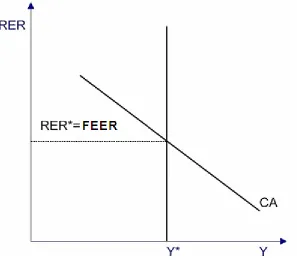
The equilibrium real exchange rate associated with internal and external balance is illustrated
in figure 1. The internal equilibrium condition, defined as non-inflationary full-employment
output, is given by the vertical schedule at the full-employment income point (Y*)8 in the
real income (Y) and real exchange rate (R) space. The external balance condition, defined as
a targeted level of the current account balance, is given by the downward sloping current
account (CA) schedule. The schedule has a negative slope for reasons that imports rise with
an increase in income, which, in order to maintain unchanged current account position, has
to be off-set by exchange rate depreciation9, stimulating exports. The point at which the two
7 For a more thorough discussion on hystereis effects on FEER, see Wren-Lewis (1992), Bayoumi et al. (1994),
Wren-Lewis and Driver (1998)
8 According to Bayoumi et al. (1994), the full-employment level of income and the full-employment level of
output will be approximately the same.
curves intersect, i.e. when both the internal and external balance conditions are met, gives
[image:19.612.158.455.148.413.2]the FEER (R*).
Figure 1: FEER, the exchange rate consistent with internal and external balance
Source: Bayoumi et al. (1994, 24)
The traditional approach to estimating the FEER inspires from the process of calculating the
PPP equilibrium exchange rate – it involves identifying a base period in which the exchange
rate is assumed to have been in equilibrium and then extrapolating that exchange rate. This
approach, however, has two deficiencies – the arbitrary choice of the base period, and the
assumption that the FEER has remained constant. Instead, it would be more appropriate to
calculate the FEER as the exchange rate that would be consistent with the economy being in
equilibrium (Williamson, 1983).
Two approaches to estimating the FEER can be found in the literature. The first one, the
general equilibrium, or the model based approach, is based on a macro-econometric model,
already existing or specially estimated, on which the internal and external balance conditions
are imposed, and which is then solved for the real exchange rate, the FEER. Three studies
Williamson (1983) calculates the FEER for the US dollar, the Japanese yen, the German
mark, the Pound sterling and the French franc for 1976-1977 and extrapolates them to 1983,
using the IMF’s Multilateral Exchange Rate Model. The external equilibrium condition is
imposed as the current account target for the five countries set on the ground of the actual
current account balances, the long-term net capital outflows and the savings and
investments; the internal balance condition is imposed as the cyclically normal demand. He
then calculates the FEERs for the five currencies for 1976-1977, and extrapolates them to
1983 by considering the factors that might have affected the FEER in the interim.
Bayoumi et al. (1994) illustrate how the FEER10 can be estimated on the example of the G-7
currencies in the early 1970s, i.e. the break-up of the Bretton-Woods system, using the IMF’s
Multimod model. Due to the illustrative nature of their study, they impose the external
balance as a current account of 1% of GDP, and the internal balance as IMF’s estimates of
the output gap.
Coudert and Couharde (2002) use the NIESR’s NIGEM11 model to estimate the FEER for
the Czech Republic, Poland, Hungary, Slovenia and Estonia for 2000 and 2001. The internal
balance is imposed as the trend output obtained using the Hodrick-Prescott filter, and the
external balance as values of the current account taken from Doisy and Herve (2001) for the
first four countries, and from Williamson and Mahar (1998) for Estonia.
One clear advantage of this approach is that it is consistent, as all the feedbacks are taken
into account. Additionally, as Wren-Lewis and Driver (1998) state, there is no need to worry
about the meaning of the medium term, as models produce projections for any period in the
future. Also, hysteresis effects are taken into account. The main disadvantage of this
approach is connected with the difficulty of building a macro-econometric model.
Furthermore, the quality of the FEER estimates obtained using the model based approach
10 Actually, Bayoumi et al. (1994) estimate the Desired Equilibrium Exchange Rate (DEER), but it is
conceptually identical to the FEER
11 NIESR=National Institute for Economic and Social Research, NIGEM=National Institute’s Global
depends critically on the quality of the model used. Finally, these estimates may lack
transparency, i.e. it might be difficult to isolate factors behind different FEERs (Wren-Lewis
and Driver 1998).
However, as Wren-Lewis (1992) notes, the process of estimating the FEER is in principle a
comparative static, partial equilibrium calculation. In the second approach, based on a partial
equilibrium, unlike in the model-based approach, the FEER is calculated by modelling only
the external sector, i.e. the current account, not the whole economy. The internal and
external balance conditions are established in the same manner as in the model based
approach, when exogenous estimates of the trend output and the current account balance
are fed into the model.
Wren-Lewis and Driver (1998) estimate the FEERs for the G-7 countries for 1995 and 2000
using the partial equilibrium approach. They model the current account as a sum of the
balance of goods and services, the interest, profit and dividend flows, and the net transfers.
The trade is split between goods and services, exports and imports, volumes and prices.
Trade volumes are modelled as a demand curve, as a function of demand and
competitiveness. They use two estimation methods for obtaining the trade elasticities – the
Johansen technique and the Error Correction Model. Goods prices are modelled as a
function of commodity prices, domestic prices and world export prices, while consumer
prices, domestic for exports and OECD for imports, are taken as the price of the services.
The interest, profit and dividend flows are modelled as a function of domestic assets,
external liabilities, real exchange rate and the interest rate for the credits and the debits, while
net transfers are modelled as a function of an intercept term and a deterministic trend. The
current account targets for the external balance criterion are taken from Williamson and
Mahar (1998), and the trend output estimates are taken from Giorno et al. (1995).
Costa (1998) estimates the FEER for the Portuguese economy for the 1980-1995 period.
Following Dolado and Vinals (1991) she uses one equation model of the fundamental
account, where the fundamental account is the sum of the current account and the net
structural capital flows. For the net structural capital flows she takes the net direct
direct investments abroad). The fundamental account is then modelled as a function of the
domestic demand, the foreign demand, the degree of openness of the economy and the real
effective exchange rate. As in the medium term the current account equals the structural
capital flows, the external balance condition is imposed as a zero fundamental account, while
the internal balance by using the trend value of the explanatory variables, obtained by the HP
filter.
Genorio and Kozamernik (2004) estimate the FEER for the Slovenian economy for the
1992-2003 period modelling the current account as the difference between export and
import values, the latter being modelled as a product of volumes and prices. Export and
import prices are taken at their trend values, obtained by a non-linear trend and the HP filter.
Trade volumes are modelled as a function of demand, competitiveness and the terms of
trade; they use 6 alternative specifications of the trade model; the model is estimated by the
OLS method. The external equilibrium is set as the current account target; they use 4
alternative current account targets. The internal equilibrium is imposed by the trend values
of the explanatory variables, obtained by the exponential trend, except in the case of the
terms of trade, where the trend values are obtained by the HP filter and the non-linear trend.
A slightly modified approach to estimating the FEER can be found in Faruqee et al. (1999);
the difference is in the treatment of the external balance condition. They model the
savings-investment relationship, and obtain the structural current account position via a quantitative
assessment, instead of imposing it in a judgemental manner. They model the underlying
current account in a similar manner to the previously mentioned studies, and calculate the
FEER as the exchange rate that equalises these two.
An application of this approach on the case of Macedonia can be found in Gutierrez (2006).
She estimates the underlying current account using the non-oil trade volumes equations from
Isard et al. (2001), and the structural current account using the equation for developing
countries, excluding Africa, from Chinn and Hito (2005). The use of these equations is the
point at which this study can be criticised most, as such panel estimations do not account for
the specificities of the individual countries, and therefore, the equations used may not be
The comparative static approach has certainly got its advantages. Its merits include simplicity
and clarity. It does not require a model of the whole economy. Additionally, factors standing
behind different levels of FEER are not difficult to identify, and sensitivity analysis to
different assumptions can be easily conducted. However, the simplicity has a price.
As Wren-Lewis (1992) and Wren-Lewis and Driver (1998) point out, the demand curve
modelling of the trade, traditional to the FEER calculations, has several shortcomings. The
first line of criticism stresses the neglect of non-price competitiveness factors. Second, the
activity variable used in the calculation is the natural rate output, which is by definition
independent of demand considerations, while imports and exports depend entirely on
demand. While this might be valid for intermediate goods, for final goods some measure of
final demand is more appropriate. Finally, the most serious criticism is that the traditional
demand curve way of modelling trade does not take into account supply-side factors.
Another problem is the exogenous treatment of the trend output and the capital flows,
ignoring any feedbacks that FEER might have on them (see Wren-Lewis and Driver, 1998).
Additionally, the structural capital flows and the trend output, being both exogenous inputs
in the calculation, may not be mutually consistent, which would not be a problem had they
been independent (Wren-Lewis and Driver, 1998). Finally, the dependence of the level of
FEER on the adjustment path towards it, i.e. the hysteresis of the FEER, is not accounted
for in the partial equilibrium approach to calculating FEER.
However, the costs of the simplification do not seem to be disastrous. Wren-Lewis and
Driver (1996) conclude that the effects of feedbacks from the real exchange rate to output
are relatively small. Wren-Lewis et al. (1991) obtain similar estimates for the UK’s FEER
using both model based and partial equilibrium approach. Bayoumi et al. (1994) obtain that
in many cases the FEER estimates for the G7 countries using the two approaches do not
differ by more than 10 percent for any country. These findings seem to provide enough
CHAPTER 3
Estimating the FEER of the denar
In this chapter the partial equilibrium approach to estimating FEER explained in the
previous chapter is applied in order to calculate the FEER of the Macedonian denar. The
chapter is structured in the following way - after the model is explained in the first section,
the data are discussed in the second. The implementation of the model is explained in the
next three sections: first the trade equations are estimated; then the trend values of the
exogenous inputs are obtained; finally a range of FEER estimates is obtained. The chapter is
concluded with a discussion on the drawbacks of the study.
3.1. Methodology
As was mentioned in the previous chapter, the process of estimating the FEER consists of
imposing internal and external balance conditions on a model, and solving it for the real
effective exchange rate.
The methodology adopted here derives from Wren-Lewis and Driver (1998) and Genorio
and Kozamernik (2004). It differs from Wren-Lewis and Driver (1998) in that our study
models the trade volumes but not the prices; it differs from Genorio and Kozamernik (2004)
in that they identify the current account with the trade account, i.e. they exclude the debt
interest flows and the net current transfers from the current account model, while this study
does not.
The current account is modelled as a sum of the trade flows, the net transfers and the debt
interest flows, following Wren-Lewis and Driver (1998). The demand approach to modelling
trade, as suggested by Goldstein and Khan (1985) is employed, where trade depends on
demand (domestic and foreign activity) and competitiveness (real effective exchange rate).
The trade is modelled as a difference between export and import values; values are modelled
The internal balance condition is imposed when values corresponding to the equilibrium are
substituted for the exogenous inputs (domestic and foreign activity, debt interest flows and
net transfers); the external balance condition is imposed as the targeted current account to
which the sum of the trade flows, the net transfers and the debt interest flows is equalised.
The model is:
int + tran + trade =
CA (1)
M * Pm -X * Px =
trade (2)
RER) f(Yf, =
X (3)
RER) f(Yd, =
M (4)
CA standing for the current account, ‘trade’ for the trade flows, ‘tran’ for the net transfers,
‘int’ for the debt interest flows, X and M for exports and imports volumes, respectively, Px
and Pm for exports and imports prices, respectively, Yf and Yd for foreign and domestic
activity, and the bar denoting the equilibrium values of the variables.
The two trade equations are first estimated, in the log-linear form:
1 3
2
1+α *lnYf+α *lnRER+ε
α
=
lnX (5)
2 6
5
4+α *lnYd+α *lnRER+ε
α
=
lnΜ (6)
α2 and α3 standing for export volumes elasticities to foreign activity and the real exchange rate respectively, α5 and α6 for import volumes elasticities to domestic activity and the real
exchange rate, α1 and α4 representing the intercept terms in the equations, ε1 and ε2
representing the error terms, and ln denoting the natural logarithm.
Assuming: RER ln * α + Yf ln * α + α = X
ln 1 2 3 (7)
RER ln * α + Yd ln * α + α = Μ
i.e. that the equilibrium export and import volumes are obtained when equilibrium values for
the activity variables and the exchange rate are substituted in the estimated trade equations,
equation (1) can be rewritten as:
int + tran + e
* Pm -e
* Px =
CA [α1+α2ln( Yf)+α3ln(RER )] [α4+α5ln( Yd)+α6ln(RER )]
(9)
The FEER is then found as the solution for RER in equation (9). As there is one unknown
and one equation, there is a unique solution; however, this exponential equation cannot be
solved by the standard analytical methods, but must be solved iteratively. One of the
methods is by using the Newton-Raphson algorithm (Monahan, 2001)12.
Therefore, three stages can be identified in the process of calculating the FEER. First, the
trade equations, i.e. equations (5) and (6) are estimated. Then the equilibrium values of the
exogenous inputs (Px,Pm,Yf,Yd,tran,int) are obtained. Finally, the FEER is calculated, i.e.
equation (9) is solved for RER .
3.2. Data
The data used in the analysis is presented in Appendix 1. The sample spans from 1998q1 to
2005q3, giving 31 observations. It is driven by the availability of data on Macedonian export
and import prices, which are not available for the periods before or after.
Data on Macedonian export and import volumes are obtained when export and import
values are divided by export and import prices, respectively. Trade values data are from
IMF’s International Financial Statistics (IFS), in dollars, nominal; trade prices data are from
National Bank of the Republic of Macedonia (NBRM), index numbers. Data on the real
12 The Newton-Raphson algorithm is an iterative algorithm for approximating a root of a function. It starts
with a number close to the solution, x0, and uses the following algorithm for calculating the iterations:
) x ( f
) x f( -x = x
n '
n n 1 +
n (10)
Where f stands for the function and f’ for its first derivative.
The solution is found when xn and xn+1 get close enough to each other (Monahan, 2001).
In our case, the function is equation (9), the conversion was set at 6 decimal places, and for xo the value of the
effective exchange rate (REER) are from IMF’s IFS, index numbers; rise in the REER
represents real appreciation, i.e. fall in price competitiveness.
The domestic activity variable is Macedonian GDP by 1997 prices, treated as real GDP,
from the National Statistical Office of the Republic of Macedonia (NSORM). The foreign
activity variable, following Genorio and Kozamernik (2004), is constructed as a weighted
average of the imports of the major 13 trading partners, using the weights obtained when
Macedonian exports to those 13 countries for the whole period are normalised to 1.
Countries who participate with more than 1,5% in the Macedonian exports for the period
were included as major trading partners. These 13 countries account for 87% of the
Macedonian exports (see Table 1). Data on Macedonian exports by countries are from the
NBRM, nominal, in dollars. Imports data for all the countries are from the IFS, except data
for Serbia and Montenegro, which are from the National Bank of Serbia. They are all
nominal, in dollars, and are converted into real using import prices, wherever possible,
otherwise using US’s PPI (Serbia and Montenegro, Croatia, Slovenia and Bulgaria13). Import
13 The decision to use the US PPI as a deflator when nominal trade was converted into real was a necessity, but
is, arguably, the best approximation, as can be seen from the analysis below.
The data we have (А) is the nominal trade (trade values) converted into dollars using the nominal exchange rate in the current period; the data we need is the trade volumes, i.e. real trade, R. Let us denote with N the nominal trade, with Pd and Pf domestic and foreign price levels, respectively, with ER the nominal exchange rate, and let
the indices c and b after Pd,Pf and ER stand for the base and the current period, respectively. Then:
A=N*ERc (11)
c
ER A =
N (12)
Assuming the real trade is given when the nominal is corrected for the change in the domestic price levels, i.e.
dc db P P * N =
R (13)
and substituting (12) into (13), we have:
c dc
db ER * P
P * A =
R (14)
пrices and US’s PPI data are from IFS, index numbers. Data on net transfers and debt interest flows are from the NBRM, nominal, in dollars, and are deflated using the US PPI.
dc fb db fc db dc fb fc b c P * P P * P = P P P P = ER
ER (15)
Rearranging (15) we get:
fb fc b db dc c P P * ER = P P *
ER (16)
Substituting (16) into (14) we obtain:
b fc fb ER 1 * P P * A =
R (17)
ERb and Pfb are constants, and, consequently, cancel out when the numbers are converted into index numbers.
Therefore, to obtain R we just need to divide A, i.e. the data we have, with the foreign price index. As all the values are in US dollars, we use US price index. We choose the PPI instead of the CPI as studies (see Breuer, 1994) have shown that the PPP holds more for the PPI, which consists of tradable goods.
Table 1: Structure of Macedonian exports by countries and
weights attached to each country in the construction of the foreign activity variable
Country
Macedonian exports to country, period 1998q1-2005q3,
in percents
Weight
Germany 20.10 0.23
Serbia and Montenegro 21.54 0.25
Greece 10.49 0.12
Italy 7.45 0.09
USA 7.82 0.09
Netherlands 3.18 0.04
Croatia 4.47 0.05
Switzerland 1.76 0.02
Great Britain 2.27 0.03
Slovenia 2.03 0.02
Bulgaria 2.50 0.03
France 2.21 0.03
Turkey 1.58 0.02
Total 87.40 114
3.3. Discussion about the characteristics of the Macedonian economy
Several issues emerge prior and with regards to the estimation of the trade equations. As a
common first step in any empirical analysis of time series data, the series are examined for
the order of integration. This determines the estimation technique to be used, as in time
series analysis the variables often turn out to be non-stationary and OLS estimates might
reflect spurious relationship in that case (unless the variables are cointegrated); in that case
cointegration methods are more appropriate (Harris and Sollis, 2003). Also, there have been
some important events in the period under observation, and the effects of these events must
be taken into consideration when modelling trade, as failure to do so might lead to obtaining
biased estimates. Therefore, as a corollary to the later analysis, and as an answer to the above
posed questions, we proceed with a discussion on the characteristics of the Macedonian
economy and on the behaviour of the data series in the observed period.
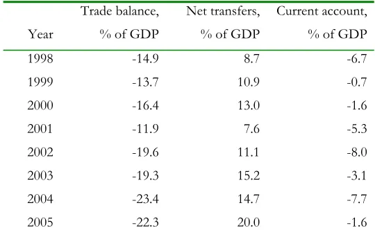
Macedonia in the observed period is characterised by continuously high trade deficits, stable
at around 14% of GDP in the period 1998-2001, and higher in the 2002-2005 period, around
and above 20% of GDP. Not much can be noticed about the current account, except that it
is negative throughout all the period. The net transfers constitute a significant part of the
current account, around 10% of GDP in the 1998-2002 period, and 15-20% of GDP in the
[image:30.612.170.440.230.401.2]2003-2005 period (Table 2).
Table 2: Trade balance, net transfers and current account, as % of GDP
Year
Trade balance, % of GDP
Net transfers, % of GDP
Current account, % of GDP 1998 1999 2000 2001 2002 2003 2004 2005 -14.9 -13.7 -16.4 -11.9 -19.6 -19.3 -23.4 -22.3 8.7 10.9 13.0 7.6 11.1 15.2 14.7 20.0 -6.7 -0.7 -1.6 -5.3 -8.0 -3.1 -7.7 -1.6 Exports, imports and current account data from IFS. Net transfers data from
the NBRM. GDP data from the NSORM.
Bearing in mind that intermediate products represent a majority of imports, i.e. about
60-65% (NBRM 1998-2005), a high elasticity of imports with respect to domestic activity can be
expected a priori. Due to the high level of dependency of the economy on imports, one
would expect only moderately high exchange rate elasticity of imports. On the exports side,
fairly high exchange rate elasticity can be expected, as the majority of exports consist of
products from the commodity end of the market, about 45-55% (NBRM 1998-2005). Taking
into account the small size of Macedonia relative to the world, one would not expect high
world activity elasticity of exports.
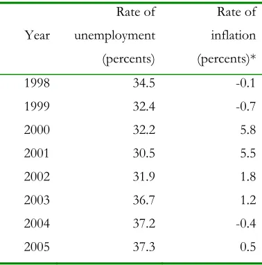
In the period under examination the Macedonian economy is characterised by extremely
high unemployment rates and low inflation rates. Table 3 summarises these data. The higher
higher inflation in 2001 was a consequence of the psychological effect of the crisis, which
[image:31.612.211.400.145.336.2]caused a depreciation in the nominal exchange rate.
Table 3: Unemployment and inflation rates
Year
Rate of unemployment (percents)
Rate of inflation (percents)* 1998
1999 2000 2001 2002 2003 2004 2005
34.5 32.4 32.2 30.5 31.9 36.7 37.2 37.3
-0.1 -0.7 5.8 5.5 1.8 1.2 -0.4 0.5
*Inflation measured by consumer prices Source: NSORM (1998-2005)
The period observed is characterized by two external shocks. The first one is the conflict in
FR Yugoslavia in the first half of 1999 and the accompanying refugees crisis in Macedonia;
the second one is the conflict in Macedonia in the first, second and third quarter of 2001.
The effects of both shocks on Macedonian import volumes can be seen from Figure 2 – dramatic fall in the first two quarters of 1999 and in the first three quarters of 2001. The
1999 shock caused a fall in the export volumes in the first half of 1999, while the immediate effects of the 2001 shock on the exports are disguised by the fall in export prices (Figure
4)15; however, the prolonged effects of the crisis are clear – a structural break in the first
quarter of 2002, characterised by a fall in the intercept (Figure 3). The effects of the first
crisis on economic activity are evident – fall in the first two quarters of 1999, while the effects of the second crisis are not that clear (Figure 5).
15 Although the fall in the export prices instead of in the export volumes in 2001 is quiet surprising,
Figure 2: Macedonian import volumes, 1998-2005
1998Q1 1998Q4 1999Q3 2000Q2 2001Q1 2001Q4 2002Q3 2003Q2 2004Q1 2004Q4 2005Q3
Figure 3: Macedonian export volumes, 1998-2005
1998Q1 1998Q4 1999Q3 2000Q2 2001Q1 2001Q4 2002Q3 2003Q2 2004Q1 2004Q4 2005Q3
Figure 4: Macedonian export prices, 1998-2005
Figure 5: Macedonian GDP, 1998-2005
1998Q1 1998Q4 1999Q3 2000Q2 2001Q1 2001Q4 2002Q3 2003Q2 2004Q1 2004Q4 2005Q3
We also present the plots of the other series used in the analysis – the foreign demand
variable (Figure 6) and the real effective exchange rate (Figure 7), as a support to the formal
unit root tests presented in the next section16.
Figure 6: Foreign demand, 1998-2005
1998Q1 1998Q4 1999Q3 2000Q2 2001Q1 2001Q4 2002Q3 2003Q2 2004Q1 2004Q4 2005Q3
16 We believe that it is a good practice to examine each data series ‘by eye’, prior to conducting all the formal
Figure 7: Real Effective Exchange Rate of the denar
1998Q1 1998Q4 1999Q3 2000Q2 2001Q1 2001Q4 2002Q3 2003Q2 2004Q1 2004Q4 2005Q3
3.4. Tests of order of integration of the series
The order of integration of the series plays crucial role in the empirical analysis, since the
decision on the estimation method is driven by it. A few common tests were applied in order
to determine the order of integration of the series – the Augmented Dickey-Fuller (ADF)
test, the ADF Generalised Least Squares (ADF-GLS) test, the ADF-Perron method and the
Philips-Perron (PP) test. When the ADF test was done, the Dolado-Enders sequential
testing procedure was followed (Enders, 1995), and the results presented are those on which
the decision of rejection or otherwise of the null was based. The ADF-GLS test uses
Generalised Least Squares detrending, and is characterised by a greater power and better
performances in small samples than the other tests (Harris and Sollis, 2003). The
ADF-Perron test allows for structural break in the series (ADF-Perron, 1989), and is used for the export
volumes series, since the structural change is suspected there. The PP test is similar to the
ADF test, with that difference that it uses non-parametrical statistical methods to account
for a possible serial correlation, i.e. it uses Newey-West adjusted standard errors, which are
robust on heteroskedasticity and serial correlation. The caveat with the PP test is that the
Newey-West S.E.’s are a large sample technique. We, however, report this test. As the
weaknesses of the tests are well acknowledged in the literature (low power and size, poor
not rely on any particular test but, rather, assemble an evidence base using all appropriate
[image:35.612.87.527.135.481.2]tests17. Table 4 presents these tests.
Table 4: Results of the test of the hypothesis that the series are non-stationary
Series ADF test ADF-GLS test ADF-Perron PP test Decision
Export volumes
Not rejected on any
level*
Not rejected on any
level
Rejected on
all levels
Not rejected on
any level
Ambiguous. Either
non-stationary or
stationary with break
Import volumes
Not rejected on 1%
Rejected on 5%
and 10%*
Not rejected on any
level
Not rejected on
1%. Rejected on
5%
Non-stationary
Foreign Demand
Not rejected on any
level **
With 4 lags, rejected
on 5% and 10%, not
on 1%
Not rejected on
any level without
trend.
Not-rejected on
1%, rejected on
5% with trend
Ambiguous. Either
stationary around a
deterministic trend, or
non-stationary
Domestic GDP
Not rejected on any
level***
Not rejected on any
level
Not rejected on
1%. Rejected on
5% Non-stationary Real effective exchange rate
Rejected on all
levels****
With more than 1 lag,
not rejected on any
level
With 1 lag, rejected
on 5% and 10%, not
on 1%
Not rejected on
1% and 5%,
rejected on 10%
Ambiguous, probably
non-stationary
* intercept included, as the coefficient in front of the lag of the level was higher than 1;
** 4 lags included due to serial correlation; intercept included; trend included (significant at 5%); *** 4 lags and an intercept included;
**** no constant, no trend, no lags included
Besides the ambiguity of the test results on some of the occasions, it was decided to proceed
as the series were non-stationary and, thus, appropriate for cointegration analysis. Next, tests
for unit root in the first differences of the series are conducted.
Table 5: Results of the tests for unit root in the first differences series
Series DF test ADF test ADF-GLS test PP test
Export volumes Rejected on all
levels
Rejected on all
levels
Rejected on all
levels
Import volumes Rejected on all
levels
Rejected on all
levels
Rejected on all
levels
Foreign Demand Rejected on all
levels**
Rejected on all
levels
Rejected on all
levels
Domestic GDP Rejected on all
levels*
Rejected on all
levels
Rejected on all
levels
Real effective exchange rate
Rejected on all
levels***
Rejected on all
levels
Rejected on all
levels
* the hypothesis of no serial correlation was rejected, even when lagged values of the dependent variable were included ** two lags and an intercept included
*** one lag included, due to serial correlation
The results of the tests in Table 5 are rather unanimous. The first differenced series are
stationary, therefore we proceeded as if the series are integrated of order 1 (I(1)).
3.5. Estimating the trade equations
Dealing with a sample with such a short time span (8 years), for reasons of robustness, two
estimation methods were employed for obtaining the trade equations – the Auto Regressive
Distributed Lag (ARDL) model and the Johansen technique. Another factor that influenced
the decision to use two methods for obtaining the trade equations was the wish to have
alternative trade elasticities, for sensitivity analysis purposes.
ARDL estimates
If the Johansen technique is a kind of a standard when estimating time series models, the
decision to use the ARDL method was based on the well recognised advantages of this
method - it can be applied irrespectively of whether the variables are I(0) or I(1) and it has
The ARDL method is based on estimating an Error Correction Model by the OLS method,
which, for two independent variables and two lags is of the form:
' t 1 -t 9 1 -t 8 1 -t 7 2 -t 6 1 -t 5 2 -t 4 1 -t 3 2 -t 2 1 -t 1 0 t u + Z α + X α + Y α + Z Δ α + Z Δ α + X Δ α + X Δ α + Y Δ α + Y Δ α + α = Y Δ (18)
The first part of the ECM (the lagged changes) gives the short-run dynamics, while the
second part (lagged levels) the long-run relationship.
Implementing the ARDL approach for obtaining the long-run relationship between the
variables of interest, involves two stages: first, whether there exists a long-run relationship
between the variables is tested; and second, if exists, a long-run relationship is estimated
(Pesaran and Pesaran, 1997).
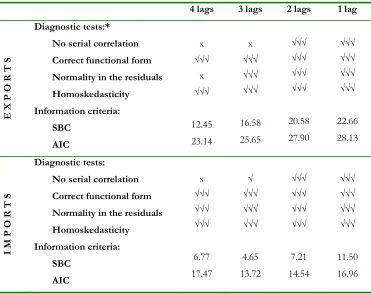
Before the existence of long-run relationship is tested, the maximum number of lags in the
ARDL has to be chosen. The decision has to balance between including enough lags so as to
ensure statistical validity and not including too many lags due to the small sample size. Two
criteria are employed for the purpose: the diagnostic tests of the regressions, as a measure of
the statistical validity; and the Schwartz Bayesian Criterion (SBC) and the Akaike
Information Criterion (AIC), as a measure of the regression-fit, where the option with the
highest value for the information criteria is chosen (Pesaran and Pesaran, 1997, 130). We
started with four lags, as a common rule when working with quarterly data, and tested down.
The results are given in Table 618.