Testing the nullity of GARCH coefficients : correction of the standard tests and relative efficiency comparisons

Munich Personal RePEc Archive

Testing the nullity of GARCH

coefficients : correction of the standard

tests and relative efficiency comparisons

Francq, Christian and Zakoian, Jean-Michel

Testing the nullity of GARCH coefficients :

correction of the standard tests and relative

efficiency comparisons

Christian Francq

and Jean-Michel Zakoïan

Abstract: This article is concerned by testing the nullity of coefficients in GARCH models. The problem is non standard because the quasi-maximum likelihood estimator is subject to positivity constraints. The paper establishes the asymptotic null and local alternative distributions of Wald, score, and quasi-likelihood ratio tests. Efficiency comparisons under fixed alternatives are also considered. Two cases of special interest are: (i) tests of the null hypothesis of one coefficient equal to zero and (ii) tests of the null hypothesis of no conditional heteroscedasticity. Finally, the proposed approach is used in the analysis of a set of financial data and leads to reconsider the preeminence of GARCH(1,1) among GARCH models.

The quasi-maximum likelihood estimator (QMLE), which is the most widely-used estimator for GARCH models, possesses a non standard asymptotic distribution when the true parameter has zero coefficients. It follows that tests currently implemented in softwares, such as the t-ratio test, the Wald test or the Likelihood Ratio (LR) test, are

∗_{Université Lille III, GREMARS-EQUIPPE, BP 60149, 59653 Villeneuve d’Ascq cedex,}

France. E-mail: [email protected], tel: 33.3.20.41.64.87

†_{CREST and GREMARS-EQUIPPE, 15 Boulevard Gabriel Péri, 92245 Malakoff}

not valid for testing that some GARCH coefficients are equal to zero. For any sequence of local parameters tending to the boundary of the parameter space at the raten1/2

, the asymptotic distribution of the QMLE is established. This allows to correct the asymptotic critical values of the above-mentioned tests and to compare their local asymptotic powers. We give conditions under which the modified versions of the Wald and LR tests are locally asymptotically optimal for testing the nullity of one coefficient, and we show that these tests dominate the usual two-sided score test. For testing that the ARCH coefficients are all equal to zero, we show that a one-sided version of the score test enjoys the property of being locally asymptotically most stringent somewhere most powerful. We also compute and compare the Bahadur slopes of several conditional homoscedasticity tests, showing that the asymptotic performance of a given test strongly depends on the efficiency concept (e.g. Bahadur or Pitman) chosen.

Keywords : Asymptotic efficiency of tests, Boundary, Chi-bar distribution, GARCH model, Quasi Maximum Likelihood Estimation, Local alternatives.

1

Introduction

GARCH coefficient. In practice, testing the nullity of parameters in the GARCH framework is achieved by applying standard tests, such as the Wald test, the Rao-score (or Lagrange Multiplier) test and the Likelihood Ratio test. These standard tests are provided by most standard time series packages currently available for GARCH estimation (e.g. GAUSS, RATS, SAS, SPSS).

Unfortunately, as we will see, this common practice may be based on an invalid asymptotic theory. Tests in GARCH models have received much less attention than the theory of estimation. Despite its apparent simplicity, the problem of testing that some coefficients are equal to zero in a GARCH model is non trivial. The reason is that the Quasi Maximum-Likelihood Estimator (QMLE) is positively constrained. It follows that the standard distributions for some widely used tests are not asymptotically valid.

The primary objective of this paper is to derive asymptotically valid critical values for the Wald, Rao-score and Quasi-Likelihood Ratio (QLR) statistics. Given the variety of possible tests we decided to limit ourselves to the most widely used procedures. Our second goal is to compare the efficiencies of those tests under fixed and local alternatives. We will use the approximate Bahadur slope criterion and the Pitman analysis for power comparisons.

The most important cases for applications are: (i) tests of the null hypothesis of one coefficient equal to zero and (ii) tests of the null hypothesis of no conditional heteroscedasticity. In these two special cases, detailed asymptotic efficiency (local and non local) comparisons can be done. For the nullity of one coefficient, the widely used Student’s test will be also considered. A special attention will be given to testing conditional homoscedasticity. In this case we will also compare the three general tests with the Lee and King (1993) test, which exploits the one-sided nature of the alternatives and enjoys optimality properties.

which, under the null hypothesis, the parameter is at the boundary of the main-tained assumption. Such problems have been considered e.g. by Chernoff (1954), Bartholomew (1959), Perlman (1969), Gouriéroux, Holly and Monfort (1982). Sev-eral papers consider one-sided alternatives. These include Wolak (1989), Rogers (1986), Silvapulle and Silvapulle (1995), King and Wu (1997); see the latter pa-per for further references. Other papa-pers on tests focus on ARCH or GARCH models. Andrews (2001) considered testing conditional homoscedasticity against a GARCH(1,1) model. This testing problem, involving a nuisance parameter un-der the null, is not consiun-dered in the present paper. The one-sided nature of the ARCH models entails positive autocorrelations of the squares at all lags, resulting in a spectral mode at frequency zero. Hong (1997) and Hong and Lee (2001) pro-posed tests for ARCH effects using spectral density estimators at frequency zero of a squared regression residual series. Dufour et al. (2004) used Monte-Carlo tests techniques which do not rely on asymptotic results. Tests of ARCH(1)-type effects in autoregressive processes, possibly with unit root, have been considered by Klüppelberg, Maller, van de Vyver and Wee (2002). Lee and King (1993), which will be directly used in the present paper, and Demos and Sentana (1998), who considered similar testing problems, will be commented later on.

requires an extension of FZ estimation results to the case of local alternatives to a parameter at the boundary.

The article is organized as follows. Section 2 presents the estimation results, in particular when the true parameter value is on the boundary, and the main test statistics. Section 3 determines their asymptotic null distributions. Section 4 establishes the asymptotic distribution of the QMLE under sequences of local alternatives to the null parameter value. Section 5 uses these results to compare the local powers of the tests. Efficiency comparisons in the sense of Bahadur are also considered. Sections 6 and 7 apply these results to the two main examples: testing the nullity of one coefficient and testing the absence of ARCH effect. Section 8 is devoted to an application to financial time series in which the preeminence of the GARCH(1,1) model is reconsidered. Section 9 concludes. Proofs are relegated to an appendix.

If a matrixA_{is semi-positive definite, a semi-norm of a vector} x_{of appropriate} dimension is defined by _kx_kA = (x′Ax)1/2. The notation a =c b will stand for

a = b +c. For a vector x_{, inequalities such as} x _{> 0 or} x _{≥ 0 have to be} understood componentwise. Let δ0 denote the Dirac mass at 0 and χ2k the chi-square distribution with k degrees of freedom. The mixture of δ0 with probability

p andχ2_k with probability 1₋p will be denoted by pδ0+ (1−p)χ2k.

2

Model and test statistics

Assume that the observed time series ǫ1, . . . , ǫn is generated by the GARCH(p, q) model







ǫt=√htηt

ht=ω0+Pq_i=1α0iǫ2t−i+

Pp

j=1β0jht−j, ∀t∈Z

where θ0 := (ω0, α01, . . . , α0q, β01, . . . , β0p) is a parameter vector and the noise sequence (ηt)is iid with mean 0 and variance 1. Under the positivity constraints

ω0>0, α0i ≥0 (i= 1, . . . , q), β0j ≥0 (j= 1, . . . , p),

Bougerol and Picard (1992) showed that a uniquenonanticipative strictly stationary solution (ǫt) exists if and only ifγ(A0)<0where, for any normk · k on the space

of the (p+q)_×(p+q) matrices, γ(A_{0) = limt→∞} 1

tlogkA0tA0,t−1. . .A01k a.s. and

A_0t=



        

α01:q−1η2t α0qηt2 β01:p−1ηt2 β0pηt2

I_{q−1 0 0 0}

α01:q−1 α0q β0p−1 β0p

0 I_{p−1 0}



        

with α01:q−1 = (α01. . . α0q−1), β01:p−1 = (β01. . . β0p−1) and Ik being the k×k identity matrix. A nonanticipative solution (ǫt) of Model (1) is such that ǫt is a measurable function of the ηt−i, i≥ 0. Note that Nelson and Cao (1992) derived necessary and sufficient conditions for the positivity of the volatility process σ2_t. However these conditions are not very explicit and thus seem difficult to use for statistical purposes.

The primary objective of this article is to develop a methodology for testing the nullity of a sub-vector ofθ0. More precisely, and without loss of generality we

consider testing the nullity of the lastd2coefficients ofθ0, split into two components

asθ₀= (θ(1)₀ ,θ(2)₀ )′, whereθ(₀i) _∈Rdi_,d

1+d2 =p+q+ 1 =d.The null hypothesis

is thus

H0 : θ(2)0 =0d2×1 i.e. Kθ0 =0d2×1 with K=

0_d

2×d1, Id2

denote our maintained assumption. To proceed, we define the vector of param-eters as θ = (θ1, . . . , θp+q+1)′, with θ1 = ω, and the parameter space Θ as any

compact subset of [0,_∞)p+q+1 _{that bounds the first component away from zero.}

For technical reasons we also assume that Θcontains some hypercube of the form [ω, ω]_×[0, ε]p+q_{, for someε >0 and ω > ω >0.}

To define the QMLE, the initial values are, for simplicity, taken equal to zero, i.e. ǫ2

0=. . . =ǫ21−q= ˜σ02=. . . = ˜σ21−p= 0, and the variablesσ˜2t(θ)are recursively defined, for t≥1, by

˜

σ_t2(θ) =ω+ q

X

i=1

αiǫ2t−i+ p

X

j=1

βjσ˜2t−j.

A QMLE of θ is defined as any measurable solution ˆθn of θˆn= arg minθ_∈Θ˜ln(θ),

where˜ln(θ) = n−1Pn

t=1ℓ˜t, and ℓ˜t = ˜ℓt(θ) = ˜ℓt(θ;ǫn, . . . , ǫ1) =

ǫ2 t

˜

σ2

t + log ˜σ

2

t. An ergodic and stationary approximation (σ2

t(θ)) of the sequence (˜σ2t(θ)) is ob-tained as follows. Under the strict stationarity condition γ(A_{0) < 0 and if}

Pp

j=1βj <1,denote by σt2

=

σ_t2(θ) the strictly stationary, ergodic and nonan-ticipative solution of σ_t2 = ω +Pq

i=1αiǫ2t−i +

Pp

j=1βjσt2−j, for all t. Note that σ2_t(θ0) = ht. Let Aθ(z) =

Pq

i=1αizi andBθ(z) = 1−

Pp

j=1βjzj.By convention, Aθ(z) = 0 if q= 0 and Bθ(z) = 1if p= 0. Under the conditions

A1: θ0∈

◦

Θwhere Θ◦ denotes the interior of Θ,

A2: γ(A_{0)<0 and} Pp

j=1βj <1, ∀θ∈Θ,

A3: η2

t has a non-degenerate distribution withEηt2 = 1 andκη =Eηt4 <∞,

A4: ifp >0,_Aθ₀(z) andBθ₀(z) have no common root,Aθ₀(1)6= 0, andα0q+ β0p6= 0,

Eθ₀

1

σ4 t(θ0)

∂σ2 t(θ0) ∂θ

∂σ2 t(θ0) ∂θ′

is well-defined and the QMLE is asymptotically normal:

√

n(ˆθn−θ0)→ NL 0,(κη −1)J−1 , κη =Eη4t. (2)

A1 is a standard assumption for the asymptotic normality, but in the GARCH framework it constrains the coefficients to be positive. It is important to note thatA2-A4 are sufficient for the strong consistency. In A2, the strict stationarity condition is imposed only at the value θ0. For all other parameter values, it is

sufficient to make the given assumption on the βi coefficients. Assumptions A3 and A4 are made for identifiability reasons.

The usual forms of the Wald, Rao-score and QLR statistics follow, and are given by

Wn = n ˆ κη −1

ˆ

θ(2)

′

n

n

KˆJ−_n1K′

o−1

ˆ

θ(2)_n ,

Rn = n ˆ κ_η|2−1

∂˜lnˆθn|2

∂θ′ Jˆ

−1

n|2

∂˜ln

ˆ

θn|2

∂θ ,

Ln = n

n

˜ln

ˆ

θ_n|2−˜ln

ˆ

θn

o

,

where θˆ_n|2 denotes the restricted (by H0) estimator of θ0, ˆκη,κˆη|2 denote

consis-tent estimators of κη, andJˆn,ˆJn|2 denote consistent estimators of the information

matrix J_{. In general,}Jˆ_{nand ˆκη are derived using the unconstrained estimatorθ}ˆ_n, whereas Jˆ_{n|2 and κˆη|2 are computed using θ}ˆ_{n|2. For instance, one can take}

ˆ J_n= 1

n n X t=1 1 ˜ σ_t4(ˆθn)

∂σ˜_t2(ˆθ_n) ∂θ

∂σ˜_t2(ˆθ_n)

∂θ′ , Jˆn|2=

1 n n X t=1 1 ˜ σ_t4(ˆθn|2)

∂˜σ2_t(ˆθ_n|2) ∂θ

∂σ˜2_t(ˆθ_n|2) ∂θ′ ,

and

ˆ κη =

1 n

n

X

t=1

ǫ4_t ˜ σ_t4(ˆθn)

, κˆη|2 =

1 n

n

X

t=1

ǫ4_t ˜ σ4_t(ˆθn|2)

,

because

1 Xn ǫ2_t

= 1 n

X ǫ2_t

Note that the latter equalities imply that

Ln= 1 n

n

X

t=1

logσ˜

2

t(ˆθn|2)

˜

σ_t2(ˆθn) , a.s.

One rejects the null hypothesis for large values of Wn,Rn,Ln. In the next section, we give the asymptotic distributions of these statistics under the null hypothesis.

3

Non standard asymptotic null distributions

FZ underlined that, among the assumptions required for the asymptotic normality (2), A1 is quite restrictive since it implies θ0 >0 componentwise. Indeed if, say,

θ0i = 0, the variable √n(ˆθni−θ0i) = √nθˆni is nonnegative and thus cannot be asymptotically normal. Note that this problem cannot be solved by blowing up the parameter spaceΘoutside the positive quadrant, since the variableσ˜2_t(θ)must be positive for the loglikelihood to be well-defined.

Thus, to obtain the asymptotic distribution of √n(ˆθn−θ0) under H0,A1 is

replaced by the following assumption. Letθ0(ε)be the vector obtained by replacing

all zero coefficients of θ0 by a number ε.

A1’: θ0(ε)∈

◦

Θfor some ε >0,where Θ◦ denotes the interior ofΘ.

AssumptionA1’, though compatible withH0, is intended to preventθ0from

reach-ing the upper bound of Θ. In some cases, no moment assumption on the observed process (ǫt) will be required. In other cases a moment condition is necessary. The following two assumptions will be made alternately.

A5: Eθ₀ǫ6_t <∞,

A6: {j |β0,j >0} 6=∅ and j0

Y

i=1

Note thatA6 does not cover the ARCH case, where all theβ0i coefficients are equal to zero. LetΛ =Rd1_×[0,∞)d2_{.The following result displays the asymptotic} distri-bution of the QMLE and of the score vector∂ln(θ0)/∂θwhereln(θ) =n−1Pnt=1ℓt, and ℓt=ℓt(θ) =ǫ2t/σt2+ logσ2t.

Theorem 1 (Francq and Zakoian, 2007) IfH0,A1’,A2–A4and either A5or

A6 hold, √

n(ˆθn−θ0) →d λΛ:= arg inf

λ_∈Λ{λ−Z}

′_{J{λ−Z}, Z∼ N}

0_,(κη−1)J−1 _, √

n∂ln(θ0) ∂θ

d

→ N {0_,(κη−1)J_},

where in the definition of J_{, derivatives with respect to the lastd2 components are}

replaced by right derivatives.

The asymptotic distribution of the QMLE is thus non standard when the true parameter has coefficients equal to zero, but it can be easily simulated. Note that λΛ can be interpreted as the projection of Z_{, for the metric defined by} J_, onto the convex set Λ = _{λ _∈ Rd _| K_{λ ≥} 0_{}. The faces of Λ are sections of} the subspaces {λ _∈ Rd _| K_{iλ =} 0_{}, where the} K_{i are obtained by cancelling} 0, 1 or several rows of K_{. Projecting} Z _{onto those subspaces yields the vectors}

λK_i = PiZ, where Pi = Id −J−1K′i KiJ−1K′i

−1

K_{i. The solution is thus} obtained as

λΛ =Z_1lΛ(Z_{) + 1gΛ}c(Z)×argmin_λ

∈Ckλ−ZkJ=Z1l_Λ(Z) +

2d2₋₁

X

i=1

P_iZ_1lD

i(Z), (4)

where C ={λK_i :i= 1, . . . ,2d2 −1 andKλK_i ≥ 0} is the set of admissible

pro-jections (those with nonnegative last d2 components) and the Di form a partition of Rd_{. For instance, when all the coefficients α0i are equal to zero in an ARCH(q)} model (d1 = 1, d2 =q, d=q+ 1), it can be seen that (4) reduces to

λΛ= Z +ω d

X

Z−, Z+,· · · , Z+

!′

We are now in position to derive the asymptotic distributions of the three test statistics introduced in Section 2. Let Ω ₌ K′_(κη−1)KJ−1K′ −1K_{. Note} that for any z _{= (}z(1)_,z(2)₎′ _∈ Rd _{we have} z′Ωz _{= k}z(2)_k

{var(Z(2)_)}−1 where Z= (Z(1)_,Z(2)₎′ _{is as in Theorem 1.}

Theorem 2 UnderH0 and the assumptions of Theorem 1 we have

Wn →d W =λΛ

′

Ω_λΛ_{, (6)}

Rn →d χ2d2, (7)

Ln →d L =− 1 2(λ

Λ_−Z)′J_(λΛ₋Z_{) +}1 2Z′K′

KJ−1K′ −1KZ

= ₋1 2

inf

Kλ_≥0k

Z_−λk2_{J− inf}

Kλ=0k

Z_−λk2_J

. (8)

An interesting point is that, contrary to the standard situation, the asymptotic distributions of those statistics are not the same. Only the score statistic has the standard χ2_d2 distribution, which is a consequence of the gaussian asymptotic distribution of the score vector underH0. This implies that the standard Rao score

test remains valid whatever the position of θ0, in the interior or on the boundary

of Θ. On the contrary, valid tests based on the Wald and LR statistics require correction of the usual critical values. This problem is well known in situations where the parameter is constrained both under the null and the alternatives (see Chernoff (1954) and the references in the introduction).

By Theorem 2, tests of asymptotic levelα are defined by the critical regions

{Wn>w1−α}, {Rn> χ2d2,1−α}, {Ln>l1−α}

4

Non regularity of the QMLE under local

al-ternatives

For local power comparisons, the asymptotic distribution of the QMLE under sequences of local alternatives to the null parameter value θ0 is required. Let

θn =θ0+τ/√n, where τ = (τ0, . . . , τp+q)′ ∈ (0,+∞)p+q+1 is such that θn∈ Θ, at least for sufficiently large n.

We need to precisely define the data generating process. Write A_{0 =} A_(θ0) and assume that A2 holds. For n large enough, γ{A₍θ₀+τ/√n)} < 0 and we can define the nonanticipative and strictly stationary solution (ǫt,n)_t∈Z of







ǫt,n =pht,n ηt

ht,n=ω0+√τ0_n+Pqi=1

α0i+ √τi_n

ǫ2_t−i,n+Pp

j=1

β0j+τ√q+_nj

ht−j,n, ∀t∈Z

where (ηt) is iid (0,1). Given the observations ǫ1,n, . . . , ǫn,n, the QMLE satisfies

ˆ

θn= arg min

θ_∈Θ

1 n

n

X

t=1

˜

ℓt,n(θ), ℓ˜t,n(θ) = ˜ℓt(θ;ǫn,n, . . . , ǫ1,n) = ǫ2

t,n ˜ σ2

t,n

+ log ˜σ_t,n2 , (9)

where σ˜t,n = ˜σt,n(θ) is obtained by replacing ǫu by ǫu,n, 1 ≤ u < t, in ˜σt but, for simplicity, with initial values independent of n. Similarly σ_t,n2 (θ) is defined by replacing ǫu by ǫu,n,u < t, in σt2(θ). Denote byPn,τ the distribution of(ǫt,n).

Theorem 3 Let θ0 ∈ Θ and let τ ∈ (0,+∞)p+q+1. Let (ˆθn) be a sequence of QMLE satisfying (9). Then, if A2-A4 hold, θˆn → θ0, Pn,τ−a.s. as n → ∞. Moreover, if the assumptions of Theorem 1 hold then √n(ˆθn−θn)is asymptotically distributed under P_{n,τ as λ}Λ_{(τ)−τ where}

λΛ(τ) = arg inf

λ_∈Λ{λ−

Z_−τ}′J_{λ−Z_{−τ}, with} Z_{∼ N}0_{,(κη −1)}J−1 _.

lemma (see e.g. van der Vaart p 90, 1998). Because the sequence _{√n(ˆθn−

θ0)′,logLn(θ0 + τ/√n) − logLn(θ0)} is not asymptotically Gaussian,

denot-ing by Ln the likelihood function, Le Cam’s third lemma seems difficult to ap-ply. The same problem was encountered by Ling (2007). However the pre-vious theorem can be established directly. For brevity the proof of Theo-rem 3 and of several other results are not given here, but are available at http://www.amstat.org/publications/jasa/supplemental_materials..

When the true value θ0 is not on the boundary, i.e. when H0 does not hold,

λΛ(τ)₋τ =Z_{is independent ofτ.However, it is seen that underH0, the QMLE} does not converge to its asymptotic distribution locally uniformly since λΛ(τ)−τ generally depends on τ. Thus, the QMLE is regular in the interior of Θ but not on the whole parameter space (see e.g. van der Vaart p 115, 1998).

5

Power comparisons

In this section, we consider two popular efficiency measures, in order to compare the asymptotic power functions of the tests. We start by Bahadur’s (1960) approach in which the efficiency of a test is measured by the rate of convergence of its p-value under a fixed alternative H1 :θ(2)0 >0.

5.1

Bahadur slopes

Let

J_{(θ) =Eθ} 0

1 σ4_t(θ)

∂σ2

t(θ) ∂θ

∂σ2

t(θ) ∂θ′

, D_{(θ) =Eθ} 0

1 σ_t2(θ)

∂σ2

t(θ) ∂θ(2)

1₋σ

2

t(θ0)

σ_t2(θ)

.

Proposition 1 Under the alternative H1 : θ(2)0 > 0 and under A1’, A2-A4, the

approximate Bahadur slope of the Wald test is

lim n→∞−

2

nlogSW(Wn) = 1 κη−1

θ(2)₀ ′ KJ−1K′−1θ(2)₀ , a.s. (10)

Moreover, under A5 and the conditions (43), (44) and (46) discussed in the ap-pendix, the approximate Bahadur slope of QLR test is

lim n→∞−

2

nlogSL(Ln) = Eθ0 log σ2

t(θ0|2)

σ2

t(θ0)

!

, (11)

where θ_0|2 is the a.s. limit ofθˆ_n|2. If in addition D_(θ0

|2)6= 0,

lim n→∞−

2

nlogSR(Rn) = 1 κ_η|2−1D

′_(θ

0|2)KJ−_0|1₂K′D(θ0|2), (12)

where J₀

|2 = J(θ0|2) and κη|2 is the kurtosis coefficient of σ−t1(θ0|2)ǫt under H1.

It follows that the Wald, score and QLR tests are consistent, in the sense that the

probability of rejecting H0 tends to one under H1.

The term "approximate" Bahadur slopes serves to distinguish the limits in (10) and (12) from other quantities, called "exact" Bahadur slopes, which are defined by substituting the non-asymptotic survival functions for the asymptotic ones (e.g. P(Xn > t) for SW(t), where Xn is distributed as Wn under θ(2)0 = 0) in the

above definitions. We are unable to pursue the exact versions because we do not have large-deviation results for the statistics Wn, Rn and Ln. For a discussion of approximate and exact slopes, see Bahadur (1967). In the Bahadur sense, a test is considered more efficient than another one when its slope is greater. This approach is sometimes criticized (see e.g. van der Vaart (1998)) and is not easy to use in our framework because the information matrices J _and J₀

|2 are not known in closed

5.2

Pitman analysis

Whereas Bahadur’s approach considers non-local alternatives and compares the rates at which the P-values of two tests converge to zero, the Pitman approach considers sequences of local alternatives, and compares the local asymptotic pow-ers of the tests. We denote by χ2_k(c) the noncentral chi-square distribution with noncentrality parameter c and k degrees of freedom. The asymptotic distribu-tions of the 3 test statistics under the local alternatives are given in the following theorem.

Theorem 4 Under the assumptions of Theorem 3, we have

Wn →d W(τ) =λΛ(τ)′ΩλΛ(τ), (13)

Rn →d χ2d2

τ′Ω_{τ , (14)}

Ln →d L(τ) =− 1 2

λΛτ −Z−τ ′J

λΛτ −Z−τ +

κη −1

2 (Z+τ)

′Ω₍Z_+τ)

= ₋1 2

inf

Kλ_≥0k

Z_{+τ −λk}2_{J− inf}

Kλ₌₀k

Z_{+τ −λk}2_J

. (15)

It is seen that the asymptotic distribution of the Rao statistic is very different from that of the two other statistics. The following proposition establishes that the asymptotic distributions of the Wald and the rescaled Quasi-Likelihood Ratio statistics are actually the same under the null or under the local alternatives.

Proposition 2 With the assumptions of Theorems 1 or 3, Wn oP(1)

= _κˆ2

η−1Ln. Note that under non-local alternatives the Wald and rescaled Quasi-Likelihood Ratio tests might have different powers.

6

Testing the nullity of one coefficient

In this section, we are interested in testing assumptions of the form

for some giveni_{∈ {}1, . . . , q_}(orj_{∈ {}1, . . . , p_}). This is for instance the case when a GARCH(p−1, q) (or a GARCH(p, q−1)) is tested against a GARCH(p, q). In practice, the most widely used test for a simple hypothesis is the so-called t-ratio defined, in the case of (16), by

tn= ˆ αni ˆ σαˆni

(or βˆnj ˆ σ_βˆ_nj

)

with standard notations. The maintained assumption is that all other coefficients are positive, so that d2 = 1. Let Φ(·) denote the N(0,1) cumulative distribution

function, τ∗ _{= τd/σd and σ}2

d = VarZd. The critical regions of asymptotic level α and the local asymptotic powers are as follows.

Proposition 3 (a) Under (16) and the assumptions of Theorem 1, tests of

asymp-totic level α (for α≤1/2) are defined by the critical regions

{tn>Φ−1(1−2α)}, {Wn> χ21,1−2α}, {Rn> χ21,1−α}, { 2 ˆ κη −1

Ln> χ21,1−2α}.

(b) Under the assumptions of Theorem 4, the local asymptotic power of thet-ratio,

Wald and QLR tests is

lim n→∞

P_n,τ{tn>Φ−1_{(1−2α)}= lim} n→∞

P_{n,τ{Wn> χ}2

1,1−2α}

= lim n→∞

P_n,τ{ 2Ln ˆ κη−1

> χ2_1,1−2α}= 1−Φ(c1−τ∗), (17)

and that of the score test is

lim n→∞

P_{n,τ{Rn> χ}2

1,1−α}= 1−Φ(c2−τ∗) + Φ(−c2−τ∗), (18)

where c1 = Φ−1(1−α) and c2= Φ−1(1−α/2). (c) Moreover, for any τ >0,

lim n→∞

P_{n,τWn> χ}2

1,1−2α >_nlim

→∞

P_{n,τRn> χ}2

Proposition 3(c) shows that, for testing the nullity of one GARCH coefficient, the modified Wald test is locally asymptotically more powerful than the standard score test.

Now we will see that the modified Wald test enjoys optimality properties. As-sume that ηt has a density f such that ιf =

R

{1 +yf′_(y)/f(y)}2_{f(y)dy <}

∞. Note that ιf is σ2 times the Fisher information on the scale parameter σ >0 in the density family σ−1_{f(·/σ). From Drost and Klaassen (1997), Drost, Klaassen}

and Werker (1997) and Ling and McAleer (2003) it is known that, under mild regularity conditions, GARCH processes are locally asymptotically normal (LAN) with information matrix

I_{f =} ιf 4E

1 σ4

t ∂σ2_t

∂θ ∂σ_t2

∂θ′(θ0) = ιf

4J. (19) In this framework the so-called local experiments _{Ln(θ0+τ/√n),τ ∈Λ}

con-verge to the limiting gaussian experimentn_N τ,I−1 f

,τ _∈Λo(see van der Vaart (1998) for details about LAN properties and the notion of experiments). Testing K_{θ0= 0 corresponds to testing} K_{τ = 0 in the limiting experiment. Suppose that} X _isN

τ,I−1 f

distributed. From the Neyman-Pearson lemma, the test rejecting for large values ofKX_{is uniformly most powerful against the alternatives}K_{τ >0.} This optimal test has the power

π(τ) = 1−Φ



c_α−

K_τ

q

KI−1 f K′



, c_α= Φ−1(1−α). (20)

A test whose level and power jointly converge to α and to the bound in (20), respectively, will be called asymptotically optimal.

Proposition 4 Assume that ηt has a density f such that ιf exists. For testing that one GARCH coefficient is equal to zero, the modified t-ratio, Wald and QLR

tests are asymptotically optimal if and only if

f(y) = a a

Γ(a)exp(−ay

2_)|y|2a−1_{, a >0, Γ(a) =}Z ∞ 0

Table 1: Asymptotic levels in percentages of the standard Wald and QLR tests of

nominal level 5%, for testing the nullity of one coefficient.

κη 2 3 4 5 6 7 8 9 10

Standard Wald 2.5 2.5 2.5 2.5 2.5 2.5 2.5 2.5 2.5

Standard QLR 0.3 2.5 5.5 8.3 10.8 12.9 14.7 16.4 17.8

The score test is never asymptotically optimal.

To conclude this section, it is important to note that thestandardWald test{Wn> χ2

1,1−α}, and also the standard t-ratio test {tn > Φ−1(1−α)}, have asymptotic level α/2. These two tests are therefore too conservative and may lead to select too simple ARCH models. The standard QLR test _{Ln > χ21,1−α} has the same asymptotic level α/2 when κ = 3. However, when the distribution of ηt is highly leptokurtic, which seems to be the case for many financial time series, Table 1 reveals that thestandardQLR test can lead to overrejection of the null hypothesis.

7

Testing conditional homoscedaticity

In this section, we consider the case d1 = 1 with θ(1) = ω, p = 0 and d2 = q.

This case corresponds to the problem of testing the null hypothesis of no condi-tional heteroscedasticity versus an ARCH(q)alternative. We therefore consider the hypothesis

in the ARCH(q) model







ǫt =σtηt, ηt iid(0,1)

σ_t2 =ω0+Pq_i=1α0iǫ2t−i, ω >0, α0i≥0.

(23)

7.1

Some simple test statistics

In his paper introducing ARCH, Engle (1982) noted that the score test is very simple to compute. Indeed, Rn=nR2, whereR2 is the determination coefficient of the regression of ǫ2_t on a constant andǫ2_t−1, . . . , ǫ2_t−q. An asymptotically equivalent version is

R∗_n= n (ˆκ_η|2−1)2

q

X

i=1

(

1 n

n

X

t=1

(1₋ ǫ

2

t ˆ σ2

ǫ )ǫ

2

t−i ˆ σ2

ǫ

)2

=n q

X

i=1

ˆ

ρ2_ǫ2(i), (24)

whereσˆ2

ǫ =n−1

Pn

t=1ǫ2t,κˆη|2 = (nσˆǫ4)−1

Pn

t=1ǫ4t andρˆǫ2(i)is a standard estimator of the i-th autocorrelation of (ǫ2_t). The score statistic thus has the interpretation of a portmanteau statistic for checking that (ǫ2

t)is a white noise.

Another very simple test is obtained as follows. As remarked by Demos and Sentana (1998), at the point θ0= (ω0,0, . . . ,0), the information matrix J=J(θ0)

takes a simple form and we have

(κη−1)J−1 =



      

(κη +q−1)ω20 −ω0 · · · −ω0

−ω0

.. . −ω0

I_q



      

. (25)

Because (κη−1)KJ−1K′=Iq, a simple version of the Wald statistic is

W∗_n=n q

X

i=1

ˆ α2_i.

Note thatW_n∗ is not the usual Wald statistic defined in (3), which uses the estimator ˆ

local alternative distributions of Wald statistics are not affected by the choice of a consistent estimator of J_.

Lee and King (1993) proposed a test which exploits the one-sided nature of the ARCH alternative. Their test rejects conditional homoscedasticity for large values of

LKn=− √

n1′ q∂˜ln

ˆ

θ_n|2/∂θ(2)

ˆ σLK

= √ 1 nσˆLK

q

X

i=1

n

X

t=1

(ǫ

2

t ˆ σ2

ǫ − 1)ǫ

2

t−i ˆ σ2

ǫ ,

where σˆ_LK2 is an estimator of the variance of the numerator and1_{q = (1, . . . ,1)}′ _∈ Rq_{. In view of (33), (35), (36), (37) and (25) one can take}

ˆ

σ2_LK = (ˆκ_η|2−1)1′ q

n

KˆJ_n

|2K′−(KˆJn|2K′)(KˆJn|2K′)−1(KˆJn|2K′)

o

1_q

= (ˆκ_η|2−1)1′ q

n

KˆJ−1 n|2K′

o−1

1_q=q(ˆκη

|2−1)2,

withK_{= (}0_q×1,I_{q) and}K_{= (1,}0_{1×q). It follows that}

LKn= 1 √_q

q

X

i=1

√

nρˆ_ǫ2(i).

This form is not exactly the expression given in Lee and King (hereafter LK), but is asymptotically equivalent to it under the null (and under local alternatives). We will see that the LK-test enjoys some optimality properties.

7.2

Asymptotic null distributions

Proposition 5 Under (22) and A3 we have

W∗_n →d 1 2qδ0+

q

X

i=1





q

i





1 2qχ

2

i, R∗n d

→χ2_q, LKn→ Nd (0,1), (26)

where the sum denotes a mixture of independent distributions.

Demos and Sentana (1998) obtained the same result for W∗_n by means of heuristic arguments and results established by Wolak (1989) in the iid case. They wrote on page 107 that their "analysis is based on the presumption that standard results one inequality testing can be extended" to the GARCH case. Our results allow to validate this presumption.

Simulation experiments (see Table 5 of the supplemental document at the JASA supplemental materials website) of the tests based on an ARCH(2) model, show that for reasonable sample lengths (e.g. n= 100), the sizes are never very far from the theoretical ones.

7.3

Power comparisons under fixed alternatives

The next result allows to compare the efficiencies in the Bahadur sense of the "sim-ple" tests for no conditional heteroscedasticity. Let ρǫ2 denote the autocorrelation function of the process (ǫ2_t), and letκǫ=Eθ₀(ǫ4_t)/{Eθ₀(ǫ2_t)}2. The following gives

the asymptotic relative efficiencies (ARE) of the simple conditional homoscedas-ticity tests in the presence of ARCH.

ARCH(q) model (23) with E(ǫ4

t)<∞ and

Pq

i=1α0i >0. Then,

ARE(R∗/LK) := lim n→∞−

2

nlogSR(R∗n){nlim→∞−

2

nlog{1−Φ(LKn)}}−

1

= q

Pq

i=1ρ2ǫ2(i) {Pq

i=1ρǫ2(i)}2 ≥1,

ARE(R∗/W∗) := lim n→∞−

2

nlogSR(R∗n){nlim→∞−

2

nlogSW(W∗n)}−

1

=

Pq

i=1ρ2ǫ2(i)

Pq

i=1α20i ≥1,

ARE(R/W∗) := lim n→∞−

2

nlogSR(Rn){nlim→∞−

2

nlogSW(W

∗

n)}−1 = κǫ−κη

κη(κǫ−1)Pqi=1α20i ≥1,

with equalities when q= 1.

Because a test is consistent whenever its slope is positive, these conditional ho-moscedasticity tests are consistent under much more general assumptions than the ARCH(q) alternative.

Versions of tests which are asymptotically equivalent under the null and lo-cal alternatives may have different slopes. The asymptotic efficiencies derived in Proposition 1 do not coincide with those just derived for the "simple" test statistics. However, they can be evaluated by simulation. It can be seen that

θ_0|2 =





Eθ₀(ǫ2_t)

0_q×1



, J=Eθ₀(σ_t−4ZtZ′t), J0|2 ={Eθ₀(ǫ2_t)}−2Eθ₀(ZtZ′t), with Z_{t = (1, ǫ}2

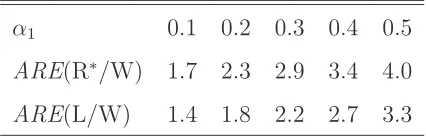
t−1, . . . , ǫ2t−q)′. The results displayed in Table 2 concern the ARCH(1), for α1 ranging from 0 to 0.4, with gaussian conditional distributions.

Note that when q = 1 the AREs computed in Proposition 6 are equal to 1. More-over, the slope of the Rao statistic given by (12) coincides with those of the other versions of the score, and is equal to α2

Table 2: Asymptotic efficiencies of the score and QLR tests relative to the Wald

test for testing conditional homoscedasticity in an ARCH(1). The number of

repli-cations of the ratio is N = 10, the expectations are evaluated by empirical means

of size 10,000,000.

α1 0.1 0.2 0.3 0.4 0.5

ARE(R∗_{/W) 1.7 2.3 2.9 3.4 4.0}

ARE(L/W) 1.4 1.8 2.2 2.7 3.3

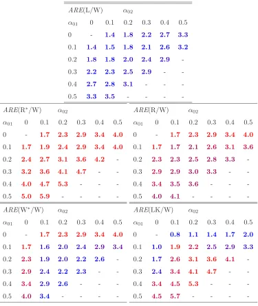
where S_≺Tmeans that a testSis less efficient thanT, andS_∼Tmeans that the two tests have the same slope. Table 3 reports efficiency results for an ARCH(2) and shows, in particular, that the equivalence observed in the caseq = 1 does not hold in general. Colors, from blue to red, indicate the rankings of those tests. To summarize, the tests can be ranked as follows

W_≺L_≺W∗ _≺R_≺R∗.

The LK cannot be ranked in general: it can have the lowest or the highest asymp-totic efficiency depending on the parameter values.

7.4

Power comparisons under local alternatives

Under mild regularity conditions, in the limiting experiment our testing problem corresponds to testing K_{τ =} 0 _{with one observation} X _{= (X1, . . . , Xq+1)}′ _∼ N(τ,I−1

f ). Let

•

τ be a point ofΛwhose lastqcomponents are equal to somec >0, and let τ◦=τ• ₋I−1

f K′(KI−f1K′)−1K

•

Table 3: Asymptotic efficiencies of conditional homoscedasticity tests relative to the Wald test, for an ARCH(2) alternative. The number of replications of the slopes is N = 10, the expectations are evaluated by empirical means of size 10,000,000. Missing values correspond to the non existence of the 4th-order moment or to α01=α02= 0.

ARE(L/W) α02

α01 0 0.1 0.2 0.3 0.4 0.5

0 - 1.4 1.8 2.2 2.7 3.3

0.1 1.4 1.5 1.8 2.1 2.6 3.2

0.2 1.8 1.8 2.0 2.4 2.9

-0.3 2.2 2.3 2.5 2.9 _-

-0.4 2.7 2.8 3.1 _{- -}

-0.5 3.3 3.5 _{- - -}

-ARE(R∗_{/W) α02}

α01 0 0.1 0.2 0.3 0.4 0.5

0 - 1.7 2.3 2.9 3.4 4.0

0.1 1.7 1.9 2.4 2.9 3.4 4.0 0.2 2.4 2.7 3.1 3.6 4.2

-0.3 3.2 3.6 4.1 4.7 _-

-0.4 4.0 4.7 5.3 _{- -}

-0.5 5.0 5.9 _{- - -}

-ARE(R/W) α02

α01 0 0.1 0.2 0.3 0.4 0.5

0 - 1.7 2.3 2.9 3.4 4.0

0.1 1.7 1.7 2.1 2.6 3.1 3.6

0.2 2.3 2.3 2.5 2.8 3.3

-0.3 2.9 2.9 3.0 3.3 _-

-0.4 3.4 3.5 3.6 _{- -}

-0.5 4.0 4.1 _{- - -}

-ARE(W∗_{/W) α02}

α01 0 0.1 0.2 0.3 0.4 0.5

0 - 1.7 2.3 2.9 3.4 4.0

0.1 1.7 1.6 2.0 2.4 2.9 3.4 0.2 2.3 1.9 2.0 2.2 2.6

-0.3 2.9 2.4 2.2 2.3 _-

-0.4 3.4 2.9 2.6 _{- -}

-0.5 4.0 3.4 _{- - -}

-ARE(LK/W) α02

α01 0 0.1 0.2 0.3 0.4 0.5

0 - 0.8 1.1 1.4 1.7 2.0

0.1 1.0 1.9 2.2 2.5 2.9 3.3

0.2 1.7 2.6 3.1 3.6 4.1

-0.3 2.4 3.4 4.1 4.7 _-

-0.4 3.4 4.5 5.3 _{- -}

-values of

(X_−τ•₎′I_f(X_−τ•₎₋₍X_−τ◦₎′I_f(X_−τ◦_{) = 2τ}•′ K′₍KI−1

f K′)−1KX+constant.

Since by (19) and (25),

KI−1

f K′ = 4ι−f1(κη−1)−1Iq, (27)

it is easy to see that this test rejects for large values of Pq+1

i=2Xi. This test is therefore uniformly most powerful to test τ1=· · ·=τq= 0 versus τ1 =· · ·=τq> 0. Similarly it can be shown that the tests which are somewhere most powerful (SMP) in Λ_\(0,_∞)_{× {}0_}q _{reject for large values ofd}′X _withd _∈[0,∞)q+1 _and Kd _{6= 0. Such a test is uniformly most powerful for testing τ1 = · · · = τq = 0} versus τ =cd_{,c >0. Of course, an optimal test in the "direction"} d _{may have a} very low power in other directions. The test rejecting for large values ofPq+1

i=2Xiis however most stringent somewhere most powerful (MSSMP) (the reader is referred to Shi (1987), Shi and Kudô (1987)1 and the references therein for the concept of MSSMP and SMP test). In view of (27), this MSSMP test has the power

π(τ) = 1₋Φ



c_α−

Pq

i=1τi

q

4qι−_f1(κη−1)−1



, c_α= Φ−1(1−α). (28)

The following corollary gives the local asymptotic powers of the conditional ho-moscedasticity tests considered in this section, and shows that the LK test is locally asymptotically MSSMP (Lee and King (1993) exhibit another optimality property for their test). The concept of locally asymptotically MSSMP test has been proposed by Akharif and Hallin (2003) in order to cope with one-sidedness in hypothesis testing.

Proposition 7 Under the local alternatives Hn(τ), τ >0, and the assumptions of Theorem 3 with p= 0, d1= 1 andd2=q, we have

λΛ(τ) = (Z1+τ1) +ω

d

X

i=2

(Zi+τi)−,(Z2+τ2)+,· · ·,(Zd+τd)+

!′

, (29)

where Z_{∼ N}0_,(κη−1)J−1 _{and (κη−1)}J−1 _{is given in (25). Thus, the local} asymptotic power of the modified Wald, score and LK tests are given by

lim

n→∞P{Wn>w1−α} = P ( _q

X

i=1

(Ui+τi)21l{Ui+τi>0} >w1−α

)

lim n→∞P

Rn> χ2q,1−α = P

(

χ2_q q

X

i=1

τ_i2

!

> χ2_q,1−α

)

lim

n→∞P{LKn> cα} = 1−Φ

cα−

Pq

i=1τi √_q

, (30)

where U_{= (U1, . . . , Uq)}′ _{∼ N(}0_,I_q).

Under the assumptions of Proposition 4, the LK test is asymptotically MSSMP

(in the sense that the right-hand side of (30) is equal to the upper bound π(τ)

defined by (28)) if and only if the density f of ηt belongs to the class defined by (21).

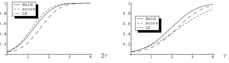
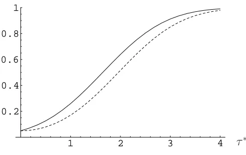
It is well known that there exists no satisfactory notion of optimality for testing hypothesis on multidimensional parameters. The LK test is asymptotically optimal in the direction α1 = · · · = αq, but there is no objective reason to favour this direction. As shown in Figure 1, the local asymptotic power of LK test may be lower than that of the Wald test, and even lower than that of the score test.

1 2 3 4 0.2

0.4 0.6 0.8 1

LK score Wald

1 2 3 4

0.2 0.4 0.6 0.8 1

LK score Wald

2τ τ

Figure 1: Local asymptotic power of the Wald, score and LK tests for testing

conditional homoscedasticity with an ARCH(2) model where α1 = α2 = τ /√n

(left figure) and α1=τ /√n, α2= 0 or α1 = 0, α2=τ /√n(right figure).

size. The asymptotic superiority of the one-sided LK test, when the alternative is symmetric in the ARCH coefficients, is reflected in finite samples. However, when the alternative is not symmetric, the LK test can be much less powerful than its competitors, both asymptotically and in finite samples. For this reason it cannot be recommended to practitioners.

8

Application: should GARCH(1,1) be

univer-sally used ?

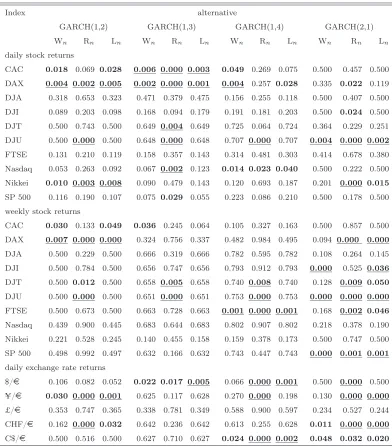
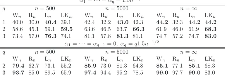
The data of this section consist of daily and weekly returns of a set of 10 indexes, namely the CAC, DAX, DJA, DJI, DJT, DJU, FTSE, Nasdaq, Nikkei, and SP500, and of 5 exchange rates. The samples extend from January 2, 1990, to March 25, 2008, for the daily stock market returns, from January 2, 1980, to March 24, 2008, for the weekly stock market returns (except for the indices for which such historical data do not exist) and from January 2, 1999, to March 31, 2008, for the exchange rates. Descriptive statistics not reported here, show that the autocorrelations for the squares are highly significant but that the return series do not display significant autocorrelations. The GARCH(1,1) model is chosen as the benchmark model and is tested, successively, against the GARCH(1,2), the GARCH(1,3), the GARCH(1,4) and the GARCH(2,1). In each case, the three tests of this paper are applied. The empirical p-values of the Wald, score and LR tests are displayed in Table 4. This table indicates that: 1) the results of the tests highly depend on the alternative, 2) the p-values of the three tests can be quite different, 3) for most of the series, the evidence is strong against the benchmark GARCH(1,1) model. Points 1) and 2) are not surprising if one admits that the data generating process (DGP) is probably neither the GARCH model of the null, nor one of the alternatives. Due to the positivity constraints, it is possible (see for instance the DJU returns) that the fitted GARCH(1,2) model satisfiesαˆ2= 0with

∂˜l_n(ˆθn

|2)/∂α2 >>0. In such a situation, where the estimate is at the boundary

A6 quite plausible. An assumption which we cannot verify is the existence of Eη_t4. An extension of the paper by Hall and Yao (2003) to the case where some coefficients are equal to zero would allow to handle the situation where Eη4

t =∞, but this is left for future research.

This study leads us to suggest the use of several tests and several alternative models. Adopting the conservative Bonferroni procedure (rejecting if the minimal p-value multiplied by the number of tests is less than a given levelα), one rejects the GARCH(1,1) null hypothesis for 16 series among the 24 series considered in Table 4. Procedures which are less conservative than Bonferroni’s approach could be applied (see e.g. Wright, 1992), but without changing the overall conclusion: the notion that the GARCH(1,1) model is sufficient for financial data can be misleading.

The R code used to produce Table 4, as well as comple-mentary illustrations and detailed proofs of technical results, can be downloaded from the JASA supplemental materials website at http://www.amstat.org/publications/jasa/supplemental_materials.

9

Concluding remarks

Table 4: p-values for tests of the null hypothesis of a GARCH(1,1) model for

stock market and change rate returns.

Index alternative

GARCH(1,2) GARCH(1,3) GARCH(1,4) GARCH(2,1)

Wn Rn Ln Wn Rn Ln Wn Rn Ln Wn Rn Ln

daily stock returns

CAC 0.018 _0.069 0.028 0.006 0.000 0.003 0.049 _{0.269 0.075 0.500 0.457 0.500}

DAX 0.004 0.002 0.005 0.002 0.000 0.001 0.004 _0.257 0.028 _0.335 0.022 _0.119

DJA 0.318 0.653 0.323 0.471 0.379 0.475 0.156 0.255 0.118 0.500 0.407 0.500 DJI 0.089 0.203 0.098 0.168 0.094 0.179 0.191 0.181 0.203 0.500 0.024 _0.500

DJT 0.500 0.743 0.500 0.649 0.004 _{0.649 0.725 0.064 0.724 0.364 0.229 0.251}

DJU 0.500 0.000 _{0.500 0.648} 0.000 _{0.648 0.707} 0.000 _0.707 0.004 0.000 0.002

FTSE 0.131 0.210 0.119 0.158 0.357 0.143 0.314 0.481 0.303 0.414 0.678 0.380 Nasdaq 0.053 0.263 0.092 0.067 0.002 _0.123 0.014 0.023 0.040 _{0.500 0.222 0.500}

Nikkei 0.010 0.003 0.008 _{0.090 0.479 0.143 0.120 0.693 0.187 0.201} 0.000 0.015

SP 500 0.116 0.190 0.107 0.075 0.029 _{0.055 0.223 0.086 0.210 0.500 0.178 0.500}

weekly stock returns

CAC 0.030 _0.133 0.049 0.036 _{0.245 0.064 0.105 0.327 0.163 0.500 0.857 0.500}

DAX 0.007 0.000 0.000 _{0.324 0.756 0.337 0.482 0.984 0.495 0.094} 0.000 0.000

DJA 0.500 0.229 0.500 0.666 0.319 0.666 0.782 0.595 0.782 0.108 0.264 0.145 DJI 0.500 0.784 0.500 0.656 0.747 0.656 0.793 0.912 0.793 0.000 _0.525 0.036

DJT 0.500 0.012 _{0.500 0.658} 0.005 _{0.658 0.740} 0.008 _{0.740 0.128} 0.009 0.050

DJU 0.500 0.000 _{0.500 0.651} 0.000 _{0.651 0.753} 0.000 _0.753 0.000 0.000 0.000

FTSE 0.500 0.673 0.500 0.663 0.728 0.663 0.001 0.000 0.001 _0.168 0.002 0.046

Nasdaq 0.439 0.900 0.445 0.683 0.644 0.683 0.802 0.907 0.802 0.218 0.378 0.190 Nikkei 0.221 0.528 0.245 0.140 0.455 0.158 0.159 0.378 0.173 0.500 0.747 0.500 SP 500 0.498 0.992 0.497 0.632 0.166 0.632 0.743 0.447 0.743 0.000 0.001 0.001

daily exchange rate returns

$/¤ _{0.106 0.082 0.052} 0.022 0.017 0.005 _0.066 0.000 0.001 _0.500 0.000 _0.500

¥/¤ 0.030 0.000 0.001 _{0.625 0.117 0.628 0.270} 0.000 _{0.198 0.130} 0.000 0.000

£/¤ _{0.353 0.747 0.365 0.338 0.781 0.349 0.588 0.900 0.597 0.234 0.527 0.244}

CHF/¤ _0.162 0.000 0.032 _{0.642 0.236 0.642 0.613 0.255 0.628} 0.011 0.000 0.000

and local alternatives; iv) the usual Rao test remains valid for testing a value on the boundary, but looses its local optimality properties;

For the two special cases considered in this paper, the approaches of Bahadur and Pitman allow efficiency comparisons, and shed light on the relative merits of the different tests. For the nullity of one coefficient, the modified Wald and QLR tests are locally asymptotically optimal, when the conditional density belongs to a class which is not restricted to the standard Gaussian. For the absence of conditional heteroscedasticity, several simple tests can be used, which have different powers under fixed alternatives. Efficiency comparisons for the ARCH(1) and ARCH(2) models suggest that the different versions of the score test are preferable to the other competitors in the Bahadur ARE sense. However, inverse conclusions are drawn when the local approach is adopted. Indeed, the score test appears to be locally dominated by the equivalent Wald and QLR tests. The one-sided version of the score test proposed by Lee and King enjoys optimality properties, but only for alternatives in certain directions. A simple version of the Wald test, rejecting the null when the sum of the squared coefficients is large, can be recommended for testing for ARCH. From both local and non local points of view, our theoretical study and numerical experiments suggest that the behavior of this test is always close to the optimum.

A ppendix: Two technical proofs

A.1

Proof of Theorem 2

The convergence in distribution (6) is a direct application of the continuous map-ping theorem, since √nˆθ(2)

′

n = K √

n(ˆθn−θ0) →L KλΛ under H0 by Theorem

1.

We now turn to the proof of (7). Sinceθˆ(1)_n|2is a consistent estimator ofθ(1)₀ >0, we haveθˆ(1)_n|2 >0fornlarge enough. Therefore∂˜lnˆθn|2

/∂θi = 0fori= 1, . . . , d1,

or equivalently

∂˜ln

ˆ

θn|2

∂θ =K

′∂˜ln

ˆ

θn|2

∂θ(2) . (31)

A Taylor expansion yields

√

n∂˜ln(ˆθn|2) ∂θ

oP(1)

= √n∂ln(θ0) ∂θ +J

√

nθˆ_n|2−θ0

. (32)

The last d2 components of this vector relation give

√

n∂˜ln(ˆθn|2) ∂θ(2)

oP(1)

= √n∂ln(θ0) ∂θ(2) +

KJ√_n

ˆ

θ_n|2−θ0

, (33)

and the first d1 components give

0 oP₌(1) √_n∂ln(θ0) ∂θ(1) +

KJK′√_n

ˆ

θ(1)_n|2−θ(1)₀

, (34)

using

ˆ

θ_n|2−θ0=K′

ˆ

θ(1)_n|2−θ(1)₀ . (35)

In view of (34), we have

√

nθˆ(1)_n|2−θ₀(1)oP=(1)₋KˆJ_n

|2K′

−1√

n∂ln(θ0)

Using (31), (33), (35) and (36) we obtain

Rn =

n ˆ κ_η|2−1

∂ln(ˆθn|2)

∂θ(2)′

KˆJ−1 n|2K′

∂ln(ˆθn|2)

∂θ(2)

oP(1)

= n κη−1

∂ln(ˆθn|2)

∂θ(2)

2

KJ−1K′

oP(1)

= n

κη−1

∂ln(θ0)

∂θ(2) +

KJK′

ˆ

θ(1)_n|2−θ(1)₀

2

KJ−1K′

oP(1)

= n

κη−1

∂ln(θ0)

∂θ(2) −

KJK′

KJK′

−1 ∂l

n(θ0)

∂θ(1)

2

KJ−1K′

.

Now recall that under H0

  W₁ W₂  := r n κη−1





∂ln(θ0) ∂θ(1) ∂ln(θ0)

∂θ(2)

  d → N   

0_,J₌





J₁₁ J₁₂

J₂₁ J₂₂

     . (37)

Using KJ−1K′ ₌ J₂₂₋J₂₁J−1

11J12

−1

it follows that the asymptotic distribu-tion of Rn is that of W2−J21J−111W1

′

J₂₂₋J₂₁J−1

11J12

−1

W₂₋J₂₁J−1

11W1

under H0, which follows the χ2_d2 distribution since W2 − J21J−₁₁1W1 ∼

N 0_,J₂₂₋J₂₁J−1

11J12

.

Turning to the proof of (8) and using (35) and (36), several Taylor expansions give

n˜lnˆθ_n|2

_o

P(1)

= nln(θ0) +n

∂ln(θ0)

∂θ′

ˆ

θ_n|2−θ0

+n 2

ˆ

θ_n|2−θ0

′

J

ˆ

θ_n|2−θ0

oP(1)

= nln(θ0)−n

2

∂ln(θ0)

∂θ(1)′

KJK′−1 ∂ln(θ0)

∂θ(1) , (38)

nln

ˆ

θn

_oP(1)

= nln(θ0) +n

∂ln(θ0)

∂θ′

ˆ

θn−θ0

+n 2

ˆ

θn−θ0

′

J

ˆ

θn−θ0

. (39)

By subtraction,

Ln oP(1)

= −n

1 2

∂ln(θ0)

∂θ(1)′

KJK′

−1 ∂l

n(θ0)

∂θ(1)

+ ∂ln(θ0) ∂θ′

ˆ

θn−θ0

+1 2

ˆ

θn−θ0

′

J

ˆ

θn−θ0

Under H0, by showing √n





∂ln(θ0) ∂θ

ˆ

θn−θ0



 →L 



−JZ

λΛ



 it can be seen that the

asymptotic distribution of Lnis the law of

L =₋1 2Z′J′K

′_J−1

11KJZ+Z′J′λΛ−

1 2λ

Λ′

J_λΛ_.

Now, because

J′K′J−1

11KJ=J−(κη−1)Ω with (κη−1)Ω=





0 0

0 J₂₂₋J₂₁J−1

11J12



,

the conclusion easily follows from

L = ₋1

2Z′JZ+ 1

2Z′(κη −1)ΩZ+Z′J′λ

Λ₋ 1

2λ

Λ′

J_λΛ

= ₋1 2(λ

Λ_−Z)′J_(λΛ₋Z_{) +} κη−1

2 Z′ΩZ. (41)

A.2

Proof of Proposition 1.

Under H1 we have limn→∞Wnn = κη1−1θ

(2)′

0 KJ−1K′

−1

θ(2)₀ . Thus, (10) is ob-tained by showing that

logSW(x) ∼ logP(χ2d2 > x) x→ ∞, (42)

and noting that Wn→ ∞and limx→∞logP(χ2d2 > x)∼ −x/2 (Bahadur, 1960). The behaviour of the two other statistics is more intricate because θˆ_n|2 does not converges to θ0 under H1. Under general conditions, see White (1982),

θ_0|2 = arg min

θ_∈Θ:θ(2)=0

Eθ₀{ℓt(θ)} exists and is unique. (43)

and the QMLE θˆ_n|2 in the misspecified (by H0) model verifies, almost surely,

ˆ

For the existence, moments of order 4 are required. For the uniqueness, a necessary condition is the local identifiability of θ0|2 (see White, 1982). This is achieved in

our model because it can be shown that, for any θ_∈Θ

J_{(θ) =Eθ} 0

1 σ4

t(θ) ∂σ2

t(θ) ∂θ

∂σ2

t(θ) ∂θ′

is a positive definite matrix. (45)

Let J∗

0|2 = J∗(θ0|2) where J∗(θ) = Eθ₀

∂2_ℓ t

∂θ∂θ′(θ)

. The existence of J∗_{(θ) is} ensured when Eǫ6_t < ∞. Note that J∗_{(θ0) =} J_{(θ0) but} J∗_{(θ0|2) =6} J_{(θ0|2). It} follows from the a.s. convergence of ˆθ_n|2 to θ_0|2 that, similar to (32)-(33),

0₌√_n∂˜ln(ˆθn|2) ∂θ(1)

oP(1)

= √n∂ln(θ0|2) ∂θ(1) +

KJ∗

0|2K′

√

nˆθ(1)_n|2−θ(1)_0|2

,

and then, assuming that

KJ∗

0|2K

′

is non-singular, (46)

√

nθˆ(1)_n|2−θ(1)₀

|2

_oP(1)

= ₋(KJ∗

0|2K′)−1

√

n∂ln(θ0|2) ∂θ(1)

= −(KJ∗

0|2K

′

)−1√1 n n X t=1 1 σ2

t(θ0|2)

∂σ_t2(θ0|2)

∂θ(1) 1−

σ_t2(θ1)

σ2

t(θ0|2)

η_t2

!

.

Note that the summand is centered because θ_0|2 minimizes the limit criterion Eθ₀{ℓt(θ)}. However it is not a martingale difference. To apply a central limit

theorem, one can rely on the strong mixing properties of GARCH processes. Such properties require additional assumptions on the density of ηt (see e.g. Carrasco and Chen (2002), Francq and Zakoian (2006)) and are beyond the scope of this paper. Applying this central limit theorem we have under H1,

√

nθˆ_n|2−θ_0|2

=OP(1). (47)

Therefore √

n∂˜ln(ˆθn|2) ∂θ(2)

oP(1)

= √n∂ln(θ0|2) ∂θ(2) +

KJ∗

0|2

√

nθˆ_n|2−θ_0|2

_o

P(√n)

It follows that, using the convergence of Jˆ_n

|2 to J0|2, and ofκˆη|2 to κη|2,

Rn n

oP(1)

= 1

κ_η|2−1

∂˜ln(ˆθ_n|2) ∂θ(2)

2

KJ−1

0|2K′ oP(1)

= 1 κ_η|2−1

∂ln(θ_0|2) ∂θ(2)

2

KJ−1

0|2K′ ,

from which (12) can be deduced by application of the ergodic theorem and argu-ments already used to establish (10). Now similar to (38) and (39) we have

n˜lnˆθ_n|2 oP=(1) nln θ_0|2

+n∂ln θ0|2

∂θ′

ˆ

θ_n|2−θ_0|2

+n 2

ˆ

θ_n|2−θ_0|2

′

J∗

0|2

ˆ

θ_n|2−θ_0|2

,

nln

ˆ

θn

_oP(1)

= nln(θ0) +n

∂ln(θ0)

∂θ′

ˆ

θn−θ0

+n 2

ˆ

θn−θ0

′

J_θˆ_n−θ0.

It follows, using (47), that

Ln n

oP(1)

= ln θ0|2

−ln(θ1)

oP(1)

= Eθ₀{ℓt(θ0|2)−ℓt(θ1)},

from which (11) can be deduced, using

Eθ₀

σ_t2(θ0)

σ2

t(θ0|2)

!

= 1. (48)

The consistency of the three tests follows from the positivity of the Bahadur slopes. From (10) it is seen that, in view of the positive definiteness of J_{, the Wald test is} consistent. In (12) the positivity of the right-hand side is ensured if D_(θ0

|2) is not

equal to zero. The consistency of the QLR test follows from

−Eθ₀ log

σ_t2(θ0)

σ2

t(θ0|2)

!

≥ −logEθ₀

σ2_t(θ0)

σ2

t(θ0|2)

!

= 0,

by (48) and Jensen’s inequality, with strict inequality whenσ_t2(θ0|2)6=σt2(θ0). The

latter is a consequence of the identifiability assumptions A3-A4.

Akharif, A. and M. Hallin (2003) Efficient detection of random coeffi-cients in autoregressive models. The Annals of Statistics 31, 675–704. Andrews, D. W. K. (2001) Testing when a parameter is on a boundary

of the maintained hypothesis. Econometrica 69, 683–734.

Bahadur, R. R. (1960) Stochastic comparison of tests. The Annals of Mathematical Statistics 31, 276–295.

Bahadur, R. R. (1967) Rates of convergence of estimates and test statis-tics. The Annals of Mathematical Statistics 38, 303–324.

Bartholomew, D. J. (1959) A test of homogeneity of ordered alternatives.

Biometrika 46, 36–48. ùProbability and Measure. John Wiley, New York.

Bollerslev, T. (1986) Generalized autoregressive conditional heteroskedas-ticity. Journal of Econometrics 31, 307–327.

Bougerol, P. and N. Picard (1992) Stationarity of GARCH processes and of some nonnegative time series. Journal of Econometrics52, 115– 127.

Carrasco, M. and X. Chen (2002) Mixing and Moment Properties of

Various GARCH and Stochastic Volatility Models. Econometric The-ory, 18, 17-39.

Chernoff, H. (1954) On the distribution of the likelihood ratio. Annals of Mathematical Statistics 54, 573–578.

Demos, A. and E. Sentana (1998) Testing for GARCH effects: A one-sided approach. Journal of Econometrics 86, 97–127.

Drost, F. C. and C. A. J. Klaassen (1997) Efficient estimation in semi-parametric GARCH models. Journal of Econometrics 81, 193–221. Drost, F. C., Klaassen, C. A. J. and B. J. M. Werker (1997)

Adap-tive estimation in time-series models. Annals of Statistics 25, 786–817. Dufour, J.-M., Khalaf, L., Bernard, J.-T. and Genest, I. (2004)