MORTEZA SEDDIGHIN AND KARL GUSTAFSON
Received 9 August 2004 and in revised form 22 March 2005
We showed previously that the first antieigenvalue and the components of the first antieigenvectors of an accretive compact normal operator can be expressed either by a pair of eigenvalues or by a single eigenvalue of the operator. In this paper, we pin down the eigenvalues ofT that express the first antieigenvalue and the components of the first antieigenvectors. In addition, we will prove that the expressions which state the first antieigenvalue and the components of the first antieigenvectors are unambiguous. Finally, based on these new results, we will develop an algorithm for computing higher antieigenvalues.
1. Introduction
An operatorTon a Hilbert space is called accretive if Re(T f,f)≥0 and strictly accretive if Re(T f,f)>0 for every vectorf =0. For an accretive operator or matrixTon a Hilbert space, the first antieigenvalue ofT, denoted byµ1(T), is defined by Gustafson to be
µ1(T)= inf T f=0
Re(T f,f)
T ff (1.1)
(see [2,3,4,5]). The quantityµ1(T) is also denoted by cosTand is called the cosine ofT.
Definition (1.1) is equivalent to
µ1(T)= inf T f=0
f=1
Re(T f,f)
T f . (1.2)
µ1(T) measures the maximum turning capability ofT. A vector f for which the
infi-mum in (1.1) is attained is called an antieigenvector ofT. Higher antieigenvalues may be defined by
µn(T)= inf T f=0
Re(T f,f) T ff, f ⊥
f(1),...,f(n−1), (1.3)
Copyright©2005 Hindawi Publishing Corporation
where f(k)denotes thekth antieigenvector. In [8,9] (see also [7]), we foundµ 1(T) for
normal matrices directly, by first expressing Re(T f,f)/T fin terms of eigenvalues of Tand components of vectors on eigenspaces and then minimizing it on the unit sphere f =1. The result was the following theorem.
Theorem1.1. LetTbe annbynaccretive normal matrix. Supposeλi=βi+δii,1≤i≤m,
are the distinct eigenvalues ofT. LetE(λi)be the eigenspace corresponding toλiandP(λi)the
orthogonal projection onE(λi). For each vector f letzi=P(λi)f. If f is an antieigenvector
withf =1, then one of the following cases holds.
(1)Only one of the vectorszi is nonzero, that is,zi =1, for someiandzj =0for
j=i. In this case it holds that
µ1(T)=βi
λi.
(1.4)
(2)Only two of the vectorsziandzjare nonzero and the rest of the components of f are
zero, that is,zi =0,zj =0, andzk =0ifk=iandk=j. In this case it holds
that
zi2
=βjλj
2
−2βiλj2+βjλi2
λi2−λj2βi−βj
,
zj2
=βiλi
2
−2βjλi 2
+βiλj 2
λi 2
−λj
2
βi−βj
.
(1.5)
Furthermore
µ1(T)=
2βj−βiβiλj2−βjλi2
λj2
−λi
2 . (1.6)
In [12], we were able to extend the above theorem to the case of normal compact op-erators on an infinite-dimensional Hilbert space by modifying our techniques in [8,9] to fit the situation in an infinite-dimensional space. However, in [12] we also took a com-pletely different approach to computeµ1(T) for general strictly accretive normal
opera-tors on Hilbert spaces of arbitrary dimension. In that approach, we took advantage of the fact [11] thatµ2
1(T)=inf{x2/y:x+iy∈W(S)}for strictly accretive normal operatorsT.
Here,S=ReT+iT∗T andW(S) denotes the numerical range ofS. The result was the following.
Theorem1.2. LetTbe a strictly accretive normal operator such that the numerical range of
S=ReT+iT∗T (1.7)
is closed. Then one of the following casesholds:
(2)
µ1(T)=
2βj−βi
βiλj
2
−βjλi 2
λj2
−λi2
(1.8)
for a pair of distinct points
λi=βi+δii, λj=βj+δji, (1.9)
in the spectrum ofT.
Mirman’s [11] observation thatµ2
1(T) can be obtained in terms ofS=ReT+iT∗T
is so immediate that no proof was given in [7,11,12], or this paper where this fact is employed. So for completeness,S=ReT+iT∗T andz =1 implies numerical range element (Sz,z)≡x+iy=Re(Tz,z) +iTz2⇒µ2
1(T)=inf{x2/y:x+iy∈W(S)}.
It is both interesting and important to pinpoint the pair of eigenvalues ofT, among all possible pairs, that actually expressµ1(T) in (1.6) in case (2) ofTheorem 1.1. In the
next section we will introduce the concept of the first and the second critical eigenvalues for an accretive normal operator and show that, among all possible pairs of eigenvalues ofT, these two eigenvalues are the ones that expressµ1(T). This will help us further to
discover which pair of eigenvalues ofT expressµ2(T) and other higher antieigenvalues
ofT. Based on the properties of the first and the second critical eigenvalues ofT, we will also show that the denominators in (1.5), and (1.6) are all nonzero for this particular pair of eigenvalues. We will also show that the radicand in the numerator of (1.6) is nonzero if (1.6) expressesµ1(T).
It should be mentioned that Davis [1] first showed that for strictly accretive normal matrices, the antieigenvalues are determined by just two of the eigenvaluesT. However, quoting Davis [1, page 174] “in general normal case I’m afraid I know no simple criterion for picking out a critical pair of eigenvalues to which attention can at once be confined.” In [8,9] we implicitly answered this question, with the ordering of the eigenvalues according to their real parts and absolute values, which more or less determines which ones led to µ1(T) according toTheorem 1.1. Also we knew that an appearance of zero denominators
and undefined numerators would not represent a problem, since the convexity arguments usually lead to the determination ofµ1byλiandλjwithλi = λj.
2. The eigenvalues expressing antieigenvalues
AssumeTis a strictly accretive normalnbynmatrix with distinct eigenvaluesλi=βi+δii,
1≤i≤m. Then as noted above, we haveµ2
1(T)=inf{x2/y:x+iy∈W(S)}, whereS=
ReT+iT∗T andW(S) denotes the numerical range ofS. SinceTis normal, so isS. By spectral mapping theorem, ifσ(S) denotes the spectrum ofS, thenσ(S)= {βi+i|λi|2:
λi=(βi+δii)∈σ(T)}. SinceSis normal, we haveW(S)=co(σ(S)), where co(σ(S))
de-notes the convex hull ofσ(S). ThereforeW(S) is a convex polygon contained in the first quadrant. Throughout this paper, for convenience, we consider an eigenvalueβi+i|λi|2
A B
C
D E
F
G
Figure 2.1
βi+i|λi|2, we may refer to (βi,|λi|2) as an eigenvalue ofS. The convexity of the function
f(x,y)=x2/yimplies that the minimum of this function onW(S) is equal to the
small-est value ofksuch that a member of the family of convex functionsy=x2/ktouches just
one point of the polygon representingW(S). Obviously, if any parabola from the family y=x2/ktouches only one point ofW(S), that point should be on∂W(S), the boundary
ofW(S). Therefore to findµ21(T), first we need to identify those values ofkfor which
y=x2/ktouches only one point of∂W(S) and then select the smallest such value. The
trivial case is when a member of the family of convex functionsy=x2/ktouches∂W(S)
at a corner point such as (βi,|λi|2). If y=x2/kis the parabola that is passing through
(βi,|λi|2), then the components of this point should satisfyy=x2/k. Hence we must have
|λi|2=β2i/k, which impliesk=βi2/|λi|2. Next consider the more interesting case when a
member of the family y=x2/ktouches∂W(S) at an interior point of an edge. In this
case the parabolay=x2/kmust be tangent to that edge at the point of contact. It is clear
that such parabolas cannot be tangent to an edge of∂W(S) if that edge has a slope which is negative, zero, or undefined because the slopes of tangent lines to the right half of parabolasy=x2/kare always positive for positive values ofk. For example, inFigure 2.1
no member of the familyy=x2/kcan be tangent to edgesAG,DE, andEF. It is also clear
that no member of the family of parabolasy=x2/kcan be tangent to an edge with
posi-tive slope ifW(S) is above the line of support ofW(S) which contains that edge without having other points in common withW(S). For instance, inFigure 2.1no parabola of the formy=x2/kcan be tangent to the edgeGFat an interior point of that edge without
actually entering into the interior ofW(S). A member of the familyy=x2/kcan however
be tangent to an edge at an interior point of that edge, without having any other common point withW(S), if the slope of that edge is positive andW(S) falls below the line of sup-port which contains that edge. For example, inFigure 2.1members of the familyy=x2/k
can be tangent to edgesAB,BC, andCD, without having any other common points with W(S).
A
B
C D
5 4 3 2 1 0
x
0 5 10 15 20 25
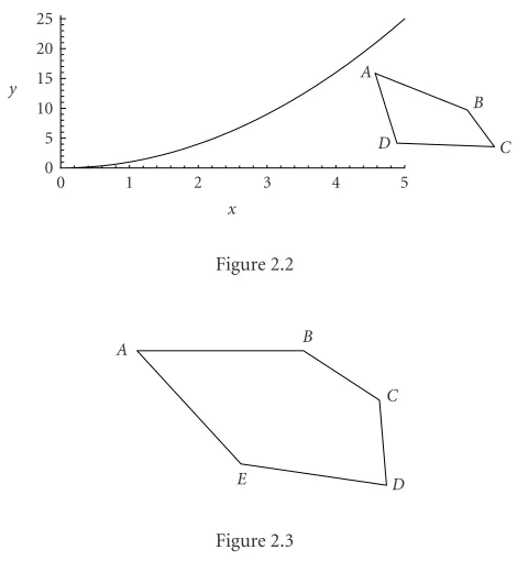
[image:5.468.116.356.67.332.2]y
Figure 2.2
A B
C
D E
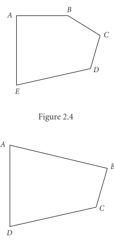
Figure 2.3
Definition 2.2. Letd=inf{βi: (βi+i|λi|2)∈σ(S)}. DefineDto be
D=supλi2:
βi+iλi2
∈σ(S),d=βi . (2.1)
Letβp+i|λp|2be that eigenvalue ofSfor whichβp=dand|λp|2=D.βp+i|λp|2is the
first critical eigenvalueγpofS. The corresponding eigenvalueλp=βp+δpiofTis called
the first critical eigenvalue ofT.
The pointAlabelling (βp,|λp|2) is shown in Figures2.2,2.3,2.4,2.5, and2.6. It
repre-sents that eigenvalue ofSwhich has the highest imaginary component among all eigen-values ofSwhich have the smallest real component.
Definition 2.3. IfA(βp,|λp|2), the first critical eigenvalue of S, is on the upper
posi-tive edgeAB andB(βq,|λq|2) corresponds to the eigenvalueγq=βq+i|λq|2 ofS, then
γq=βq+i|λq|2is called the second critical eigenvalue ofSand the corresponding eigen-valueλq=βq+δqiofT is called the second critical eigenvalue ofT. The second critical
eigenvalue ofS(ofT) is not defined ifAis not on an upper positive edge.
Theorem2.4. IfA(βp,|λp|2), the first critical eigenvalue ofS, is not on any upper positive
edge, then the minimum of the function f(x,y)=x2/yonW(S)is attained atA(β
p,|λp|2).
IfA(βp,|λp|2)belongs to an upper positive edge, then the minimum of the function f(x,y)=
x2/yonW(S)is attained at a corner point belonging to an upper positive edge or at a point
in the interior of the line segment joining the first and second critical eigenvaluesA(βp,|λp|2)
A B
C
D
[image:6.468.175.291.66.318.2]E
Figure 2.4
A
B
C
D
Figure 2.5
Proof. AssumeAB(AA1) has a positive slope. The convexity of the polygon representing
W(S) implies that if there is any set of consecutive upper positive edgesAi−1Ai, 2≤i≤
r followingAA1, then their slopes should decrease as we move from left to right. For
example, inFigure 2.1the edgeAB is followed by the edgeBCwhose slope is positive but less than the slope ofAB. AlsoBCis followed byCDwhose slope is positive but less than the slope ofBC. Suppose the slope ofAA1ism1and y=x2/k1is tangent toAA1
at a point withx-componentx1. Then we havem1=2x1/k1which impliesk1=2x1/m1.
Now suppose the slope of the segmentAi−1Ai, 2≤i≤rismiand y=x2/kiis tangent to
Ai−1Aiat an interior point withx-componentxi,then we haveki=2xi/mi. Sincem1> mi
andxi> x1, we havek1< ki.
The first critical eigenvalueA(βp,|λp|2) and the upper positive edge that containsA
(if it exists) are important in computingµ2
1(T). For example, suppose inFigure 2.2the
polygonABCDrepresents∂W(S). It is obvious that the only point of this polygon that can be touched by a member of the family of functionsy=x2/kis pointA. Depending
on the signs of the slopes of the two edges of the polygon that meet atA(βp,|λp|2), we
have two different cases that will be analyzed below.
(1)A(βp,|λp|2) does not belong to an upper positive edge. Figures2.2–2.5show the
situations when this occurs. In this case the only parabola from the familyy=x2/kthat
can touchW(S) at only one point is the one which touchesW(S) atA.
(2)A(βp,|λp|2) belongs to an upper positive edgeAB. ByTheorem 2.4 the convex
A B
C
D E
x
y
Figure 2.6
be tangent toABor pass through a corner point of an upper positive edge (see Figures
2.1and2.6).
Assume thatB(βq,|λq|2) is the higher end of the upper positive edge ABin case (2)
above.
Note that since the polygon representingW(S) is the convex hull of all eigenvalues of S, there might be other eigenvalues ofSlocated on the edgeAB. However, pointBis the end point of that edge and thus has the maximum distance from pointAamong all other points on that edge. Also note that besides eigenvalues which are located at the corners of W(S), the matrixSmay have other eigenvalues which are in the interior ofW(S). How-ever, given one such eigenvalueβi+δiithere exists pointsx+yi∈W(S) such thatx < βi
andy < βi, and hence these eigenvalues do not play any role in the computation ofµ1(T).
The first and second critical eigenvalues can be found algebraically and in practice one does not have to construct the polygon representingW(S) to find them.The procedure for findingµ1(T) is outlined in the following theorem.
Theorem 2.5. Let T be a strictly accretive normal matrix andγp=βp+i|λp|2 the first
critical eigenvalue ofS=ReT+iT∗T. Letβi+i|λi|2represent any other eigenvalue ofSfor
whichβi> βp. Letmi= |λi|2− |λp|2/βi−βp be the slopes of line segments connecting the
point(βp,|λp|2)to points(βi,|λi|2). Definem=max{mi}. Then the following two cases
hold:
(1)ifm≤0, the second critical eigenvalue ofSdoes not exist andµ1(T)=βp/|λp|,
(2)ifm >0, letR= {(βj,|λj|2) : (βj,|λj|2)σ(S)andmj=m}, and let
t=supβj−βp2+
λj2−λp2
2
:βj,λj2
R . (2.2)
If(βq,|λq|2)is that element ofR for whicht=(βq−βp)2+ (|λq|2− |λq|2)2, then
(βq,|λq|2) is the second critical eigenvalue of S. In this case µ1(T) is equal to
2(βq−βp)(βp|λq|2−βq|λp|2)/|λq|2− |λp|2 or βi/|λi| for an eigenvalueλi=βi+
Table 2.1
Point (2, 11) (3, 25) (4, 50) (5, 60)
Slope 4 9 14.333 13.25
Proof. Based on the arguments that preceded this theorem, we know that in case (1) the infimum of the function f(x,y)=x2/y on W(S) is attained at (β
p,|λp|2).
There-fore the minimum value is f(βp,|λp|2)=β2p/|λp|2. Henceµ21(T)=β2p/|λp|2, which
im-pliesµ1(T)=βp/|λp|. In case (2),Theorem 2.4shows that the minimum of the function
f(x,y)=x2/yonW(S) is attained at a corner point belonging to an upper positive edge
or at a point in the interior of the line segment joining the first and second critical eigen-values (βp,|λp|2) and (βq,|λq|2). As we just showed if the minimum of f(x,y)=x2/yon
W(S) is attained at (βi,|λi|2), we haveµ1(T)=βi/|λi|. If the minimum of the function
f(x,y)=x2/y onW(S) is attained at a point in the interior of the line segment joining
(βp,|λp|2) and (βq,|λq|2), one can use Lagrange multiplier method (see [12] for details)
to show that the point of contact is at (x1,y1), where
x1=2
βpλq2−βqλp2
λq2
−λp2
,
y1=
βpλq 2
−βqλp 2
βq−βp .
(2.3)
Therefore, in this case the minimum of the function f(x,y)=x2/yonW(S) is
fx1,y1
=x12
y1=
4βpλq 2
−βqλp
2
βq−βp
λq 2
−λp
22 . (2.4)
Thusµ21(T)=4(βp|λq|2−βq|λp|2)(βq−βp)/(|λq|2− |λp|2)2, which implies
µ1(T)=
2βq−βp
βpλq
2
−βqλp 2
λq2
−λp
2 . (2.5)
Example 2.6. Findµ1(T) ifTis a normal matrix with eigenvalues 1 +
√
6i, 2 +√7i, 3 + 4i, 4 +√34i, and 5 +√35i. First, we need to compute the corresponding eigenvalues of S=ReT+iT∗T. These eigenvalues are 1 + 7i, 2 + 11i, 3 + 25i, 4 + 50i, and 5 + 60i. The first critical eigenvalue of S is γp=1 + 7i. Thus λp =1 +√6i is the first critical
eigenvalue of T. Table 2.1 shows the slopes (or approximate values for slopes) of the line segments between the point (1, 7) and points (2, 11), (3, 25), (4, 50), and (5, 60). Since the largest slope obtained is 14.333, the second critical eigenvalue for S isγq=
4 + 50i. The corresponding second critical eigenvalue forTis therefore 4 +√34i. To find out exactly whatµ1(T) is, we need to compare the values 1/
√
7, 2/√11, 3/√25, 4/√50, 5/√60, and 2(βq−βp)(βp|λq|2−βq|λp|2)/|λq|2− |λp|2=2
(4−1)(50−28)/50−7= 2√66/43. The smallest of these numbers is 2√66/43. Hence we haveµ1(T)=2
We can indeed develop an algorithm to compute all higher antieigenvalues of a strictly accretive normal matrixT. Notice that ifTis the direct sum of two operatorsT1andT2,
T=T1⊕T2, andS=ReT+iT∗T; thenS=S1⊕S2whereS1=ReT1+iT1∗T1andS2=
ReT2+iT2∗T2. Hence, by Halmos [10, page 116], we haveW(S)=co(W(S1),W(S2)),
where co(W(S1),W(S2)) denotes the convex hull of the numerical ranges ofS1andS2. To
computeµ2(T), strike out those eigenvalues ofSthat expressµ1(T). LetE1be the direct
sum of the eigenspaces that correspond to eigenvalues which are stricken out and letE2
be the direct sum of the eigenspaces corresponding to the remaining eigenvalues. We have T=T1⊕T2whereT1is the restriction ofT onE1 andT2is the restriction ofT onE2.
Therefore,
µ2(T)=µ1T2=inf
x2
y :x+iy∈W
S2
. (2.6)
Thus, to computeµ2(T), we can replace T withT2 and computeµ1(T2) as discussed
above.
Example 2.7. Compute all antieigenvalues of a normal matrixT whose eigenvalues are 1 +√6i, 2 +√7i, 3 + 4i, 4 +√34i, and 5 +√35i. When computingµ1(T) in the previous
example we found out that the first and the second critical eigenvalues ofSare 1 + 7iand 4 + 50i, respectively, and they expressµ1(T). Hence the corresponding first and second
eigenvalues ofTare 1 +√6iand 4 +√34i, respectively. If we strike out the first and the second eigenvalues ofS, the remaining eigenvalues ofSare 2 + 11i, 3 + 25i, and 5 + 60i. The first critical eigenvalue forS2 is (2, 11). The slope of the line segment connecting
(2, 11) to (3, 25) is 14, and the slope of the line segment connecting (2, 11) to (5, 60) is 16.33. Therefore, the second critical eigenvalue ofS2is (5, 60). Henceµ2(T) is the
mini-mum of the numbers 2/√11, 5/√60, 3/√25, and 2(5−2)((2)(60)−(5)(11))/50−11= 2√195/49. The minimum of these numbers is 2√195/49. Thusµ2(T)=2√195/49. After
striking out the first and second critical eigenvalues ofS2, which expressµ1(T2), the only
eigenvalue left is (3, 25) and henceµ3(T)=3/
√ 25.
IfTis a positive matrix withndistinct eigenvaluesr1< r2<···< rn, it was proved by
Gustafson (see [2,3]) that
µ1(T)=2
√ r1r2
r1+r2.
(2.7)
In [6] Gustafson extended the notion of first antieigenvalueµ1to arbitraryA, with polar
decompositionA=UA. According to [6], the first antieigenvalue ofAis defined to be the first antieigenvalue ofA. In that caser1andr2in (2.7) are the smallest and largest
singular valuesσnandσ1ofA.
A new proof for (2.7) may be obtained within the context of this paper by clarifying thatr1andrnare the first and the second critical eigenvalues ofT, respectively.
Theorem2.8. LetTbe a positive matrix withndistinct eigenvaluesr1< r2<···< rn. Then
µi(T)=2
√ rirn−i+1
ri+rn−i+1, 1≤i≤n, (2.8)
Proof. Eigenvalues ofSarer1+r12i,r2+r22i,...,rn+rn2i. By definitionr1+ r12iis the first
critical eigenvalue ofS. To find the second critical eigenvalue ofS, we look at the slopes of line segments joining (r1,r12) to points (r2,r22), (r3,r32),...,(rn,rn2). These slopes are
(r22−r12)/(r2−r1)=r1+r2, (r32−r12)/(r3−r1)=r1+r3,...,(rn2−r12)/(rn−r1)=r1+rn.
The largest among these slopes isr1+rn which shows that (rn,rn2) is the second
criti-cal eigenvalue ofT. Thereforeµ1(T) is the minimum of the three numbersr1/
r12=1,
rn/
r2
n=1, and 2
(rn−r1)(r1rn2−rnr12)/rn2−r12=2√r1rn/r1+rn. This minimum is
obvi-ously 2√r1rn/r1+rn. The expression forµ2(T) is obtained by striking out the first and
second critical eigenvalues ofSwe just obtained and by looking at matrixS2whose
eigen-values are (r2,r22), (r3,r32), (rn−1,rn2−1). Higher antieigenvalues are obtained similarly.
3. Antieigenvalues and antieigenvectors are well defined
Now that we have pinned down which pair of eigenvalues express the first antieigenvalue µ1(T), we can restate our previous results as follows.
Theorem3.1. LetTbe annbynaccretive normal matrix. Supposeλi=βi+δii,1≤i≤m,
are eigenvalues ofT. LetE(λi)be the eigenspace corresponding toλiandP(λi)the orthogonal
projection onE(λi). For each vector f letzi=P(λi)f. Letλp=βp+δpibe the first critical
eigenvalue ofT, then one of the following cases holds:
(1)if the second critical eigenvalue ofTdoes not exist, thenµ1(T)=βp/|λp|. In this case
antieigenvectors of norm1satisfyzp =1andzi =0ifi=p,
(2)ifλq=βq+δqi, the second critical eigenvalue ofT, exists then one of the following
cases holds:
(a)µ1(T)=βi/λifor some eigenvalueλi=βi+δiiofTand antieigenvectors of norm
1satisfyzi =1andzj =0ifi=j,
(b)
µ1(T)=
2βq−βp
βpλq2−βqλp2
λq2
−λp2
, (3.1)
and antieigenvectors of norm1satisfy
zp2
=βqλq
2
−2βpλq2+βqλp2
λq2−λp2βq−βp
, (3.2)
zq2
=βpλp
2
−2βqλp2+βpλq2
λq2−λp2βq−βp
, (3.3)
andzi =0ifi=pandi=q.
In particular, the antieigenvalues and antieigenvectors are well defined.
clarify that the radicand in the expression (3.1) is nonnegative for these critical eigenval-ues. The first and second critical eigenvalues are so defined that we always haveβq> βp.
Also, by the definition of second critical eigenvalue, the slopemq=(|λq|2− |λp|2)/(βq−
βp) of the line segment between the two points (βq,|λq|2) and (βq,|λq|2) is always
pos-itive. Hence both of the termsβq−βp and|λq|2− |λp|2are positive. This implies that
the denominators in expressions (3.1), (3.2), and (3.3) are positive. Also note that the radicand in the numerator of expression (3.1) is negative ifβp|λq|2−βq|λp|2<0. In this
caseµ1(T) is not defined by (3.1). In fact, if this happens, no member of the family of the
convex functionsy=x2/kcan touch the interior of the line segment between (β p,|λp|2)
and (βq,|λq|2) since the components of such a point of contact, which are given by
ex-pressions (2.3), cannot be negative (recall thatW(S) is a subset of the first quadrant). We also need to show that the quantities on the right side of (3.2) and (3.3) are positive numbers between 0 and 1. We have already shown that the denominators of those ex-pressions are positive for the first critical eigenvalueλp=βp+δpiand the second critical
eigenvalueλq=βq+δqi. We now prove that the numerators of these expressions are also
positive for the first and second critical eigenvalues. Recall thatTheorem 3.1(2b) occurs only when a member of the family of parabolasy=x2/kintersects the line segment with
end points at (βp,|λp|2) and (βq,|λq|2) at an interior point of this segment. Therefore,
x1=2(βp|λq|2−βq|λp|2)/(|λq|2− |λp|2), which is thexcomponent of the point of
con-tact, must be betweenβpandβq. In other words
βp<2βp
λq2
−βqλp2
λq2
−λp2
< βq, (3.4)
which is equivalent to the following two inequalities:
βpλq2−βpλp2<2βpλq2−2βqλp2, (3.5)
2βpλq 2
−2βqλp 2
< βqλq 2
−βqλp 2
. (3.6)
The inequality (3.5) is equivalent to the inequalityβp|λp|2−2βq|λp|2+βp|λq|2>0.
No-tice thatβp|λp|2−2βq|λp|2+βp|λq|2is the numerator of the expression on the right side
of (3.3). Similarly, the inequality (3.6) is equivalent toβq|λq|2−2βp|λq|2+βq|λp|2>0.
Notice thatβq|λq|2−2βp|λq|2+βq|λp|2is the numerator of the expression on the right
side of (3.2). Hence the expressions on the right-hand sides of (3.2) and (3.3) are both positive. Since the sum of these two expressions is 1, each of these expressions is a number
between 0 and 1.
Since higher antieigenvalues ofT are in fact first antieigenvalues of restrictions ofT on certain reducing subspaces ofT, the higher antieigenvalues and antieigenvectors are also well defined.
To conclude, we mention that Davis’s [1, pages 173–174] theorem may not cover one instance. Thus, for clarity, we mention it here. It is possible that (using his notations)ρ= max(|λ1|/|λ2|,|λ2|/|λ1|)=1. An example isλ1= |λ1|eiθ=eiθ=cosθ+isinθ andλ2=
|λ2|e−iθ=e−iθ=cosθ−isinθ. This pair of eigenvaluesλ1andλ2cannot represent a pair
the first and second critical eigenvalues, respectively, we must haveβq> βp. Thus we are
in case (1) ofTheorem 3.1.
References
[1] Ch. Davis,Extending the Kantoroviˇc inequality to normal matrices, Linear Algebra Appl. 31
(1980), no. 1, 173–177.
[2] K. Gustafson,Positive (noncommuting) operator products and semi-groups, Math. Z.105(1968), no. 2, 160–172.
[3] , The angle of an operator and positive operator products, Bull. Amer. Math. Soc.74
(1968), 488–492.
[4] , Antieigenvalue inequalities in operator theory, Inequalities, III (Proc. 3rd Sympos., Univ. California, Los Angeles, Calif, 1969; Dedicated to the Memory of Theodore S. Motzkin) (O. Shisha, ed.), Academic Press, New York, 1972, pp. 115–119.
[5] ,Antieigenvalues, Linear Algebra Appl.208/209(1994), 437–454.
[6] ,An extended operator trigonometry, Linear Algebra Appl.319(2000), no. 1-3, 117– 135.
[7] K. Gustafson and D. K. M. Rao,Numerical Range, Universitext, Springer, New York, 1997. [8] K. Gustafson and M. Seddighin,Antieigenvalue bounds, J. Math. Anal. Appl.143(1989), no. 2,
327–340.
[9] ,A note on total antieigenvectors, J. Math. Anal. Appl.178(1993), no. 2, 603–611. [10] P. R. Halmos,A Hilbert Space Problem Book, 2nd ed., Graduate Texts in Mathematics, vol. 19,
Springer-Verlag, New York, 1982.
[11] B. Mirman,Anti-eigenvalues: method of estimation and calculation, Linear Algebra Appl.49
(1983), no. 1, 247–255.
[12] M. Seddighin,Antieigenvalues and total antieigenvalues of normal operators, J. Math. Anal. Appl.
274(2002), no. 1, 239–254.
Morteza Seddighin: Department of Mathematics, Indiana University East, Richmond, IN 47374, USA
E-mail address:[email protected]
Karl Gustafson: Department of Mathematics, University of Colorado, Boulder, CO 80309-0395, USA