Localization error estimation approaches of wireless sensor network

Localization error estimation approaches of

wireless sensor network

Venkatakrishnan.M#1, Yaashuwanth.C*2

#1

M.E Department of IT,*2Associate professor Department of IT

#1,*2

Sri Venkateswara College of Engineering, Sriperumbudur, Pin-602117, India

Abstract- The practical difficulties of setting up a wireless sensor network (WSN) and analysing its performance have made simulation essential study of WSNs. The network simulator is one of the most widely used tools by researchers to investigate the properties of WSNs. Network simulator has the basic properties to support simulations of different localization techniques. The localization algorithm calculates location accuracy and localization performance under particular level demonstrated by both Theoretical and simulation results. The enhanced performance of the proposed model calculates and compared to other algorithms using the network simulator. Results show that enhancement is obtained with the proposed algorithm when measuring metrics such as distance and localization error while varying other simulation parameters such as the number of sensors and the distance measurement error.

Keywords- Approximate Point-in-Triangulation (APIT), Distance Vector (DV), Wireless sensor networks (WSN).

I. INTRODUCTION

Location information plays a critical role in wireless sensor networks. Most of the sensor applications and techniques require that the positions of the sensor nodes be determined. Localization algorithms follow several approaches to estimate positions of sensor nodes. One approach is to use special nodes, called beacons, which know their own location, e.g. through a GPS receiver or manual configuration. More localization schemes have been developed to autonomously pinpoint the locations of normal nodes with the assistance of anchors which have perfect location information. These localization schemes fall into range based schemes or range-free schemes. Three main approaches exist to determine a node’s position: using information about a node’s neighbourhood (proximity-based approaches), exploiting geometric properties of a given scenario (triangulation and trilateration), and trying to analyse characteristic properties of the position of a node in comparison with premeasured properties (scene analysis). The common feature of range-based localization schemes is that each normal node calculates the distances or directions to the anchors or neighbours based on the following signal measurements: received signal strength, time of arrival, time difference of arrival, and angle of arrival.

II. SYSTEMMODEL

A. Approximate Point-In-Triangulation

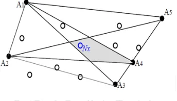
APIT algorithm does not have any specific model like circle, rectangle etc., Assume that in a network there are 5 anchors such as A1, A2, A3, A4, A5 Figure. 2.1. The concerned normal node is marked as NxThe basic principle of APIT algorithm is: Nx can

form triangles using any three anchors, as shown in Figure 1. If Nx can determine whether it is inside or outside of these

triangles, the overlap of the triangles (Nxinside) is where Nx resides. The anchors periodically broadcast beacon signals to its

neighbour nodes. In this algorithm, it is necessary for each anchor to equip with a power full transceiver, so that its signal can be received by all normal nodes in the Network. Receiving the signal from an anchor Ai each normal node detects and notes down

the received signal’s RSSI value, as well as the position of Ai.

Fig. 1 Triangles Formed by Any Three Anchors

Location estimation is performed to determine whether a normal node Nx is inside a triangle formed by three anchors.

The Perfect PIT can be performed by moving Nx along any direction, as shown in Figure. 2a. Nx moves in every possible

direction, and compares its distance to anchors with the distance before moving. The distance is measured based on RSSI. After moving a tiny step towards an every direction, Nx finds that its distance to the anchors never increase or decrease simultaneously.

Assume, when Nxmoves towards to A1, its distance to A1 becomes less, but its distances to A2 and A4both is high. Thus, Nx is

judged to be inside the triangle Δ A1 A2 A4. On the contrary, Nx will be judged outside a triangle if there is a direction such that

when Nx is moved a little, its distances to the three vertexes of the triangle increase or decrease simultaneously. For example, in

Figure 2b. When Nx moves a little, its distances to three anchors decrease simultaneously. Therefore, Nx is outside the triangle Δ

A1 A2 A3.

Fig. 2a inside ΔA1A2A4 Fig. 2b outside ΔA1A2A3

In terms of implementation, the Perfect PIT has two problems. First, it is impossible to test all directions, because there are infinite directions around the normal node N. Second, the Perfect PIT requires that normal nodes can move, however, normal nodes may be fixed in some applications. Therefore, instead of Perfect PIT, an Approximate PIT (APIT) is performed. The APIT assumes that normal nodes are static. Although normal nodes cannot move, the APIT method imagines that they could move, and regards their neighbour nodes as their positions.

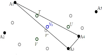
For example, as shown in Figure 3, Nxhas three neighbour normal nodes T, U and V. Like Nx these three nodes have also

received signals sent from anchors, and noted down the corresponding RSSI values. Nxcan communicate with its neighbour’s,

and obtain their RSSI values. The RSSI values are not used to calculate the exact distance, the difference between the RSSI values of two nodes is used to determine whether a node is further to an anchor than the other node.

Let us consider the triangle Δ A1 A3 A4. In order to determine whether Nxis inside the triangle, the Perfect PIT controls N to

move a very step and then observes the change of its distances to anchors. However, here, in APIT test, the static Nxvirtually

moves to its three neighbours T, U, and V. Among the three nodes (T, U, and V), Nxchecks whether there is one node that is

farther from A1, A3 and A4 simultaneously. Nx compares its RSSI value to A1 with T’s RSSI value to A1. Normally (i.e., if RSSI

values are relatively stable, not much influenced by the environment), T is closer to A1than Nx. In the same manner, it can be

tested that T is farther to A3 and A4 than Nx. So, compared with Nx, T is not farther from A1 A3 and A4 simultaneously. As for U,

the same phenomenon can be observed. If Nxhad only two neighbour nodes T and U, then through this APIT test, Nxcould have

determined that it was inside Δ A1 A3 A4.

However, in reality, Nxhas the third Neighbour V. Unfortunately, compared with Nx .V is farther from A1 A3 and A4

simultaneously. Thus, by the APIT, finally, Nxwill judge itself to be outside of the triangle, although it is actually inside the

triangle. This test error is caused by the big virtual moves in APIT test as shown in Figure 3, if V was V’, then Nx could have

determined to be inside the triangle.

Fig. 3 Example for APIT test

An overlap is formed by the triangles inside which the normal node Nxlocates. Then, the centre of this overlap is calculated as

the position of Nx. The APIT algorithm may achieve good accuracy. However, it requires anchors have high power Transmitters.

not stable. Considering these dis advantages, the APIT algorithm is rarely practiced for localization.

B. DV-Hop Localization System

The Distance Vector by Hop counting (DV-Hop) is the most known distributed algorithm. It was proposed as an ad-hoc positioning system (APS) in which sensors exchange distance vectors that contain hop counters that signifies the number of hops between the sensor receiving this vector and the sending anchor. DV-Hop assumes that every anchor i has a hop counter, Hop-Counti, and every sensor in the network stores the hop counter corresponding to every anchor; the value of the Hop-Counti

that a sensor stores about anchor i represents the minimum number of wireless hops between that sensor and the anchor i. In the first phase, an anchor i floods a message containing its ID, coordinates, and the variable Hop-Countiinitialized to zero. Sensors

store and exchange anchor hop counters.

Indeed, every time a sensor receives a message containing a Hop-Counti corresponding to an anchor i, it checks the value of the

Hop-Counti that it maintains about anchor i. If this value is less than the received one, then the latter is ignored; otherwise the

receiving sensor increments the value of the received Hop-Counti, updates its stored Hop Count, then floods it in the network. In

the second phase, anchor i computes the average hop length from its perspective, Average Hop Length, using Equation 2.1 which is given as:













2

₍

₎

)

(

i

j ij

j i i

j i j

i

Hopcount

y

y

x

x

th

Avghopleng

Where M is the number of anchors in the network, j identifies other anchors, Hop-Counti,j is the distance in hops between

anchor i and anchor j, (xi, yi) and (xj, yj) represent the coordinates of anchors i and j, respectively. After computing Average Hop

Length, anchor i flood it in the network for other anchors and sensors. A sensor maintains only the average hop length flooded by the closest anchor to it. For example where each of the three anchors A1, A2 and A3 calculates its average hop length. Then sensor node S with unknown position maintains the one that was received from A2 (i.e., the closest to S). S uses the received Average-Hop Lengthi to compute the distance dj between S and every anchor j using Equation 2.2 which is given as

j i

j

Avghopleng

th

Hopcount

d





Where, Hop Countj is the hop counter that S maintains for anchor j and Average Hop Lengthi is the average hop length that

sensor S obtained from the closest anchor, say i. In the third phase, a sensor uses the Least Square (LS) technique to trilateration its position. In basic trilateration, only three distances from anchors are necessary for an unknown sensor to find its location. The more distances available leads to better localization accuracy. The circle intersection of basic trilateration which numerically, trilateration is done by solving a system of equations.

DV-Hop localizes sensors while minimizing power consumption in the WSN, and without depending on any extra hardware. Moreover, the localization information can be used as an alternative for routing protocols to route the sensed data to the base station. The driving force behind the proposed protocol can be summarized mainly by the following three facts they are Computation and communication constraints on sensors, Perimeter deployment of anchors, Flooding phases.

Using all the calculated distances from all the anchors to be porting sensor the base station utilizes a trilateration algorithm to find the coordinates of this sensor. DV-Hop localizes sensors while minimizing power consumption in the WSN, and without depending on any extra hardware. Moreover, the localization information can be used as an alternative for routing protocols to route the sensed data to the base station. Where M is the number of anchors in the network, j identifies other anchors, Hop-Counti,j is the distance in hops between anchor i and anchor j, (xi, yi) and (xj, yj) represent the coordinates of anchors i and j,

respectively.

III.SIMULATIONRESULTS

More localization schemes have been developed to autonomously pinpoint the locations of normal nodes with the assistance of anchors which have perfect location information. These localization schemes fall into range based schemes or range-free schemes. When measuring metrics such as distance and localization error while varying other simulation parameters such as the number of sensors and the distance measurement error.

The results are based on the implementation of range free algorithms which shows the enhanced performance metrics than the existing model. The result shown below localization performance under various parameters is shown in graphs and takes the number of iterations to improve the performance metrics.

Table .1 Simulation Parameters for APIT and DV HOP system

Scenario parameters _Values

Node Radio Range

20 meters

Wireless radio propagation model

Propagation/Two ray ground

Wireless interface direction Omnidirectional

Topology area 40m×40m Square Area

Receiving power consumed 4 m-W

Anchor’s initial energy 7 k-J

Sensor’s initial energy 2 k-J

The simulation results and comparisons of the proposed system were executed and analysed using NS version 2.34 the localization performance parameters accuracy and precision estimated through various values of iterations.

Fig. 4 Localization performance graphs of distance estimation error

Figure 4 shows the comparison between the existing APIT and DV HOP and the proposed E-APIT and E-DV HOP based on parameter Hop count ratio deployed over in the sensor network. It shows that the enhancement done over the existing DV HOP model on Hop count ratio parameter.

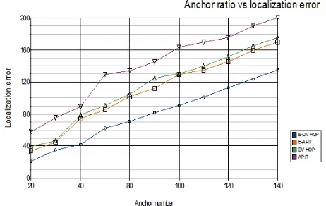
Figure 5 shows the comparison between the existing APIT and DV HOP and the proposed E-APIT and E-DV HOP based on parameter anchor ratio deployed over in the sensor network. It shows that the enhancement done over the existing DV HOP and APIT model on anchor ratio.

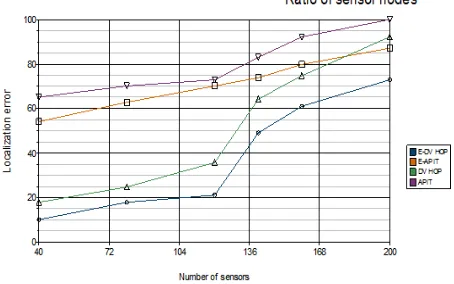
Fig. 6 Localization performance graphs of sensor ratio vs error

Figure 6 shows the performance comparison of localization system based on sensor ratio deployed over in network and localization error. It shows that the enhancement done over the existing DV HOP and APIT model on sensor ratio.

IV.CONCLUSIONS

Range free is proposed for Localization system for improving the system performance in terms of accuracy. It enhances the performance with a hardware complexity and precision complexity with respect to range free models. The simulation results and comparisons of the proposed system were executed and analysed using NS-2.34. Localization performance of range free model various values of iterations are also analysed. It was observed that the accuracy and precision performance of the system increases with the number of iteration at the cost of latency.

REFERENCES

[1] Adnan M.Abu-Mahfouz1, Gerhard P. Hancke, Sherrin J. Isaac, “Positioning System in Wireless Sensor Networks Using NS-2,” SAP journal On

Software Engineering 2012, 2(4), pp. 91-10, 2012.

[2] Baoli Zhang, and Fengqi Yu, “LSWD: Localization Scheme for Wireless Sensor Networks using Directional Antenna,” IEEE Transactions on Consumer

Electronics, vol. 56, no. 4, Nov 2010.

[3] Guangjie Han , Jia Chao , Chenyu Zhang , Lei Shu, Qing wuLi,“The impacts of mobility models on DV-hop based localization in Mobile Wireless Sensor Networks,” ELSEVIER on Journal of Network and Computer Applications 42, pp.70–79, 2014.

[4] Guang Wu, Shu Wang, Bang Wang, Yan Dong, Shu Yan, “A novel range-free localization based on regulated neighborhood distance for wireless ad hoc

and sensor networks,” ELSEVIER on Computer Networks 56 , pp. 3581–3593, 2012.

[5] Haidar Safa, “A novel localization algorithm for large scale wireless sensor networks, “ELSEVIER on Computer Communications 45, pp. 32–46, 2014.

[6] Pushpalatha.N , Anuradha.B, “Shortest Path Position Estimation between Source and Destination nodes in Wireless Sensor Networks with Low Cost,”

International Journal of Emerging Technology and Advanced Engineering, ISSN 2250-2459,vol 2, Issue 4, April 2012.

[7] Qingjun Xiao, Bin Xiao, Jian nong Cao, and Jia nping Wang, “Multi-hop Range-Free Localization in Anisotropic Wireless Sensor Networks: A