Comparison of Different De Interlacing Algorithms Using Fuzzy Logic

Comparison of Different De-Interlacing Algorithms

Using Fuzzy Logic

R. Siva1, Dr. G. Sudhavani 2 1

Communication & signal processing M. Tech, 2Professor in ECE Department, R.V.R&J.C College of Engineering, Guntur, Andhra Pradesh (522019), India

Abstract: Video processing is a special case of signal processing. These video processing techniques are used in television sets, DVDs, video players and other devices. Digital video is a representation of moving visual images in the form of encoded digital data. These video processing, which represents moving visual images with analog signals? This project can be implemented for the modern computer video displays and TV sets, which are mostly based on LCD technology. Video de-interlacing algorithms perform a crucial task in video processing. The algorithm for video de-interlacing uses the fuzzy logic to tackle two relevant features in video sequence such as motion, edges and picture repetition. De-interlacing algorithms are generally made up of two parts, such as the estimation of edge directions and the interpolation of missing pixels along with the estimated direction. This project implements a interlacing method which can detect, correct edge directions for interpolation. The Fuzzy-ELA de-interlacing method is implemented with edge-based line average (ELA) based on fuzzy logic. In this project the ELA algorithms, Fuzzy-ELA 7+7 algorithms and Fuzzy-ELA 9+9 algorithms are implemented for de-interlacing operation. The performance of these three algorithms is compared with the peak-signal to noise-ratio

Key words - Video Signal Processing, De-interlacing, Fuzzy Inference Systems, Edge adaptive line average (ELA).

I. INTRODUCTION

Fuzzy logic-based algorithms are able to model uncertainty and subjective concepts in video and image processing. Edges, for instance, are key concepts for improving the visual perception of an image. But deciding whether a pixel belongs to an edge or not is no simple task, especially if the images are noisy and/or contain a high number of details. Fuzzy logic theory provides a mathematical framework to deal with this kind of uncertain information. This study focuses on the development of fuzzy logic-based algorithms for the particular task of video processing called ‘de-interlacing’ [1]. Current digital television transmission formats use an interlaced scan mode. For example, in the popular HDTV (high-definition television) 1080i the “i” stands for interlaced scanning. Interlaced scanning is directly compatible with some CRT-based HDTV television sets on which video can be displayed natively in interlaced form, but for display on modern progressive-scan LCD and plasma TV sets, video must be de-interlaced and often scaled to the display resolution. The original version of the ELA algorithm works with 3+3 pixels from the upper and lower lines. ELA performs well when the edge direction agrees with the minimum differences of the local luminance values in the neighborhood, but otherwise introduces errors and degrades image quality. The errors usually appear when the edges are not clear, when the image is corrupted by noise, when there is a high number of details, etc. Such situations are described in this paper as areas of the picture with ‘unclear edges’. Several proposals have been presented in literature to reduce the abovementioned ELA shortcomings [3]-[10].

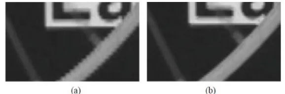
Figure 1. De-interlaced results: (a) linear versus (b) edge-adaptive algorithm.

Fuzzy inference rule bases to detect motion and to choose the most appropriate de interlacing strategy according to the degree of motion detected 19]. Used two fuzzy logic-based systems, each one tackling a feature highly relevant to de-interlacing: motion and edges. A new version of a fuzzy weighted filter capable of detecting six different edge directions was also considered [4]. The combination of a fuzzy rule-based de-interlacing algorithm and a rough sets assisted optimization algorithm [6], as well as the mixture of spatio-temporal fuzzy filters [3] were also proposed to de interlace video. The high computational costs involved in these approaches are not feasible for real time processing. Spatial de-interlaces often form part of more complex de-interlacing algorithms combining spatio-temporal interpolation. Improvements to the spatial de-interlacer therefore increase the overall performance of the spatiotemporal algorithm.

The paper is organized as follows. Section 2 describes two proposals called ‘Fuzzy-ELA 7+7’ and ‘Fuzzy-ELA 9+9’. Section 3 describes the performance of the algorithms when de interlacing a wide battery of test sequences, in comparison with other state-of the art spatial de-interlacers. Finally, some conclusions are expounded in Section 4.

II. FUZZY-ELA ALGORTHMS

A. Fuzzy-ELA 7+7 Algorithm

This algorithm looks for the most reliable edge direction and then applies line average along the selected direction. The proposed fuzzy approach applies heuristic knowledge to overcome the limitations of unclear edges. The ELA module increases the processing window up to 7+7 pixels. The ELA 7+7 algorithm considers the closest pixels to the external ends (A, G, H, N) as shown in

Figure2.

B. Rules Involved in Fuzzy-ELA 7+7 Algorithm

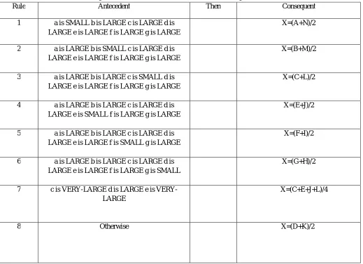
If there is a small difference in direction and a large differences in direction b, c, d, e, f and g, then an edge is clear in direction a and a linear interpolation between A and N is implemented. If there is a small difference in direction b and large differences in direction a, c, d, e, f and g, then an edge is clear in direction b and a linear interpolation between B and M is implemented.

If there is a small difference in direction c and large differences in direction a, b, d, e, f and g, then an edge is clear in direction c and a linear interpolation between C and L is implemented. If there is a small difference in direction e and large differences in direction a, b, c, d, f and g, then an edge is clear in direction e and a linear interpolation between E and J is implemented.

If there is a small difference in direction f and large differences in direction a, b, c, d, e and g, then an edge is clear in direction f and a linear interpolation between F and I is implemented. If there is a small difference in direction g and large differences in direction a, b, c, d, e and f, then an edge is clear in direction g and a linear interpolation between G and H is implemented.

If there are very large differences in directions c and e and a large difference in direction d, neither there is an edge nor vertical linear interpolation performs well; The best option is a linear interpolation between the neighbours with small differences: C, E, J, L. In other case, a vertical linear interpolation between D and K would be the most adequate.

Rule Antecedent Then Consequent

1 a is SMALL b is LARGE c is LARGE d is LARGE e is LARGE f is LARGE g is LARGE

X=(A+N)/2

2 a is LARGE b is SMALL c is LARGE d is LARGE e is LARGE f is LARGE g is LARGE

X=(B+M)/2

3 a is LARGE b is LARGE c is SMALL d is LARGE e is LARGE f is LARGE g is LARGE

X=(C+L)/2

4 a is LARGE b is LARGE c is LARGE d is LARGE e is SMALL f is LARGE g is LARGE

X=(E+J)/2

5 a is LARGE b is LARGE c is LARGE d is LARGE e is LARGE f is SMALL g is LARGE

X=(F+I)/2

6 a is LARGE b is LARGE c is LARGE d is LARGE e is LARGE f is LARGE g is SMALL

X=(G+H)/2

7 c is LARGE d is LARGE e is VERY-LARGE

X=(C+E+J+L)/4

8 Otherwise X=(D+K)/2

Table 1: Rule base of the Fuzzy-ELA 7+7 Algorithm.

III. FUZZY-ELA 9+9 ALGORITHM

a b c d e f g h i

A B C D E F G H I

X

J K L M N O P Q R

Original Pixel

Interpolated pixel

a=/ A-R/ b=/B-Q / c=/C-P/ d=/D-O/ e=/E-N/ f=/F-M/

g=/G-L/ h=/H=K/ i=/I-J/

Figure 2:Fuzzy-ELA 9+9 Algorithm

A. Rules Involved in Fuzzy-ELA 9+9 Algorithm

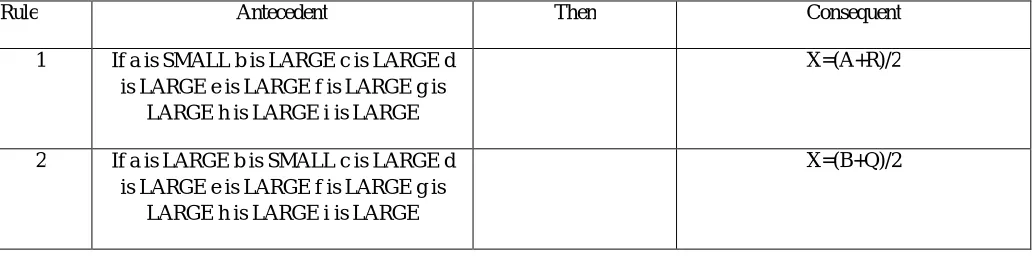
If there is a small difference in direction a and a large difference in direction b, c, d, e, f, g, h, i then an edge is clear in direction a and a linear interpolation between A and R is implemented. If there is a small difference in direction b and a large difference in direction a, c, d, e, f, g, h, I then an edge is clear in direction b and a linear interpolation between B and Q is implemented.

If there is a small difference in direction c and a large difference in direction a, b, d, e, f, g, h, i then an edge is clear in direction c and a linear interpolation between C and P is implemented. If there is a small difference in direction d and a large difference in direction a, b, c, e, f, g, h, I then an edge is clear in direction d and a linear interpolation between D and O is implemented.

If there is a small difference in direction f and a large difference in direction a, b, c, d, e, g, h, i then an edge is clear in direction f and a linear interpolation between F and M is implemented. If there is a small difference in direction g and a large difference in direction a, b, c, d, e, f, h, i then an edge is clear in direction g and a linear interpolation between G and L is implemented.

If there is a small difference in direction h and a large difference in direction a, b, c, d, e, f, g, i then an edge is clear in direction h and a linear interpolation between H and K is implemented. If there is a small difference in direction i and a large difference in direction a, b, c, d, e, f, g, h, then an edge is clear in direction i and a linear interpolation between I and J is implemented.

If there is a very large difference in direction d and f and a large difference in direction e, neither there is an edge nor does vertical linear interpolation perform well. The better option is a linear interpolation between the neighbours with small differences: D, F, M, and O. In other case, a vertical linear interpolation between E and N would be the most adequate.

Rule Antecedent Then Consequent

1 If a is SMALL b is LARGE c is LARGE d is LARGE e is LARGE f is LARGE g is

LARGE h is LARGE i is LARGE

X=(A+R)/2

2 If a is LARGE b is SMALL c is LARGE d is LARGE e is LARGE f is LARGE g is

LARGE h is LARGE i is LARGE

3 If a is LARGE b is LARGE c is SMALL d is LARGE e is LARGE f is LARGE g is

LARGE h is LARGE i is LARGE

X=(C+P)/2

4 If a is LARGE b is LARGE c is LARGE d is SMALL e is LARGE f is LARGE g is

LARGE h is LARGE i is LARGE

X=(D+O)/2

5 If a LARGE is b is LARGE c is LARGE d is LARGE e is LARGE f is SMALL g is

LARGE h is LARGE i is LARGE

X=(F+M)/2

6 If a is LARGE b is LARGE c is LARGE d is LARGE e is LARGE f is LARGE g is

SMALL h is LARGE i is LARGE

X=(G+L)/2

7 If a is LARGE b is LARGE c is LARGE d is LARGE e is LARGE f is LARGE g is

LARGE h is SMALL i is LARGE

X=(H+K)/2

8 If a is LARGE b is LARGE c is LARGE d is LARGE e is LARGE f is LARGE g is

LARGE h is LARGE i is SMALL

X=(I+J)/2

9 If d is VERY-LARGE e is LARGE and f is VERY-LARGE

X=(D+F+M+O)/4

10 Otherwise X=(E+N)/2

Table 2: Rule base of the Fuzzy-ELA 9+9 Algorithm.

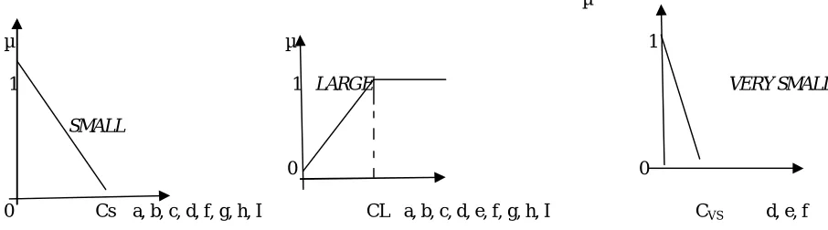
From these rules of the Fuzzy-ELA 7+7 and 9+9 Algorithms the concepts of SMALL, LARGE, VERY-LARGE are understood as Fuzzy, rather than crisp, values. This proposal translates the heuristic knowledge into fuzzy reasoning. SMALL LARGE and VERY-LARGE are represented by fuzzy sets the membership functions of which change continuously, instead of abruptly, between 0 and 1 membership values (µ) as shown in figure 3.

µ

µ µ 1

1 1 LARGE VERY SMALL

SMALL

0 0

0 Cs a, b, c, d, f, g, h, I CL a, b, c, d, e, f, g, h, I CVS d, e, f

Figure 3: Piece wise linear membership functions that employed: (a)SMALL,(b)LARGE, (c)VERY SMALL

The product operator is used as the “and” connective for antecedents to calculate the activation degree of rules from 1to 9

operator as the connective, β6 never takes negative values. Since the rule consequents (ci) are not fuzzy, the global conclusion provided by the rule base is calculated by applying the Fuzzy Mean de-fuzzification method.

Algorithm performance can be improved by tuning parameters. Shapes of piecewise linear functions in Fig. 3 were chosen heuristically, but there are many possibilities for selecting parameters that functionally describe the concepts SMALL, LARGE, and VERY_SMALL (CS, CL, and CVS). In fact, only one condition needs to be fulfilled to make the concepts SMALL and VERY_SMALL meaningful: CVS should be smaller than CS. Of the many values that meet this requirement, some will unquestionably provide better results than others. If a set of data can be obtained from progressive images, an error function can be used to evaluate the difference between using one parameter or another and supervised learning algorithms can be applied to minimize error. This is the approach that was followed to select good values for the membership function parameters.

IV. SIMULATION RESULTS

The fuzzy algorithms can simulate using the MATLAB simulation software tool. The results of the both fuzzy+ ELA Algorithms are compared as follows

(a)

(c)

Figure 4: Examples of clear edges after de-interlacing with (a) Line Average,(b) ELA 7+7, (c) ELA 9+9.

The qualitative comparison between the two proposals of the ELA algorithms can be showed as following

Figure 5: comparison between the two ELA Algorithms.

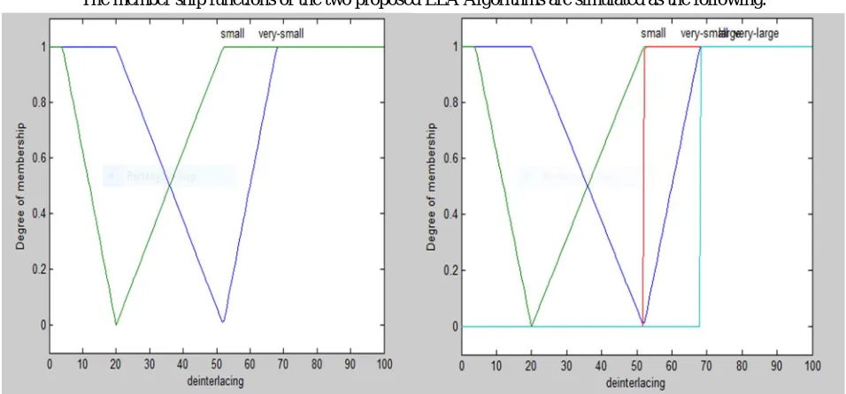
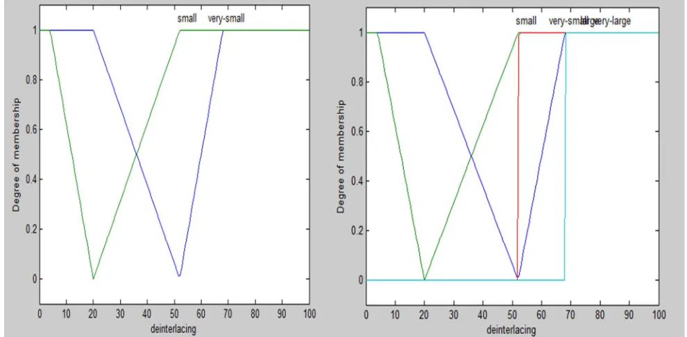
The member ship functions of the two proposed ELA Algorithms are simulated as the following.

Figure 7: Membership functions of the ELA 9+9 Algorithms.

The PSNR results of the two proposed ELA Algorithms are showed as following

Serial no Method MSE PSNR

1 LINE AVERAGE 31.24 33.18

2 FELA 7+7 DDE 17.21 35.77

3 FELA 9+9 BLI 15.81 36.14

Table 3: Comparison of PSNR value of the proposed Fuzzy ELA 7+7 Algorithm and Fuzzy of ELA 9+9 Algorithm.

IV. CONCLUSION

This paper parents two edge-adaptive de-interlacing algorithms that use fuzzy logic to detect edge directions. After extensive analysis, the conclusion is that the fuzzy-ELA 9+9 algorithm is superior to the other proposed algorithm (in terms of quantitative PSNR values and qualitative visual sensation) in both clear and unclear edges. Compared to other state-of-the-art edge-adaptive algorithms, the proposed algorithm offers a good trade-off between performance and computational cost, and there exists a strong case for its inclusion in low-cost hard ware solutions.

REFERENCES

[1] G. de Haan and E. B. Bellers, “De-interlacing - an overview,” Proceedings of the IEEE, vol. 86, no. 9, pp. 1839-1857, Sep. 1998.

[2] T. Doyle and M. Looymans, “Progressive scan conversion using edge information,” in Signal Processing of HDTV, II, Elsevier, pp. 711-721, 1990.

[3] T. Chen, H. R. Wu, and Z. H. Yu, “Efficient deinterlacing algorithm using edge-based line average interpolation,” Optical Engineering, vol. 39, no. 8, pp. 2101Aug. 2000.

[4] P.-Y. Chen and Y.-H. Lai, “A low-complexity interpolation method for deinterlacing,” IEICE Trans. on Information & Systems, vol. E90-D, no. 2, Feb. 2007. [5] M. H. Lee, J. H. Kim, J. S. Lee, K. K. Ryu, and D. Song, “A new algorithm for interlaced to progressive scan conversion based on directional correlations and

its IC design,” IEEE Trans. on Consumer Electronics, vol. 40, no. 2, pp. 119-129, May 1994.

[6] C. J. Kuo, C. Liao, and C. C. Lin, “Adaptive interpolation technique for scanning rate conversion,” IEEE Trans. on Circuits and Systems for Video Technology, vol. 6, no. 3, pp. 317-321, Jun. 1996.

[7] H. Y. Lee, J. W. Park, T. M. Bae, S. U. Choi, and Y. H. Ha, “Adaptive scan rate up-conversion system based on human visual characteristics,” IEEE Trans. on Consumer Electronics, vol. 46, no. 4, pp. 999-1006, Nov. 2000.

[9] R. Simonetti, A. P. Filisan, S. Carrato, G. Ramponi, and G. Sicuranza, “A deinterlacer for IQTV receivers and multimedia applications,” IEEE Trans. on Consumer Electronics, vol. 39, no. 3, pp. 234-240, Aug. 1993.