A comparison of two robust control techniques for throttle valve control subject to nonlinear friction

A COMPARISON OF TWO ROBUST CONTROL TECHNIQUES

FOR THROTTLE VALVE CONTROL SUBJECT TO NONLINEAR

FRICTION

Jacob L. Pedersen†, Stephen J. Dodds‡

†Delphi Diesel Systems Ltd, Park Royal, London, United Kingdom ‡CITE, University of East London, United Kingdom

[email protected], [email protected]

Abstract: Throttle valves for internal combustion engines suffer from considerable nonlinear friction in their mechanisms that is difficult to model and subject to significant variations due to changes in temperature and wear over the lifetime. The stick slip friction component is particularly troublesome. This presents a challenge to control system designers when it is important to obtain a prescribed dynamic response to reference input position changes. The contributions of this paper are a) the comparison of two different robust control techniques (sliding mode control and observer based robust control) aimed at overcoming this difficulty and b) a new simple but accurate nonlinear friction model for simulation. The control system performances using these techniques are compared with one another and with the performance attainable with a conventional PI controller.

1. Introduction:

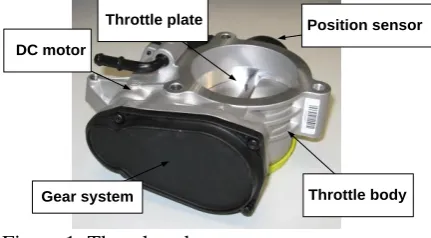
The throttle valve, an example of which is shown in Figure 1, is an essential component on both petrol and Diesel internal combustion engines. They are used mainly for controlling the air-to-fuel ratio by applying a variable constraint to the air path.

Position sensor DC motor

Throttle plate

Gear system Throttle body

Figure 1: Throttle valve

This is achieved by opening and closing the throttle plate which is driven by a DC motor through a gear system. The position is measured by a position sensor attached to the plate.

Throttle valves suffer from considerable nonlinear friction in their mechanisms that is considered difficult to model and is subject to significant variations due to changes in temperature and wear over the lifetime. The stick slip friction component is particularly troublesome and causes controller limit cycling (Armstrong-Helouvry and Amin, 1994). This presents a challenge to control system designers when it is important to obtain a prescribed dynamic response to reference input position changes.

control methods presented in this paper are intended to overcome this limitation.

2. Throttle valve modelling:

2.1 Linear throttle valve model:

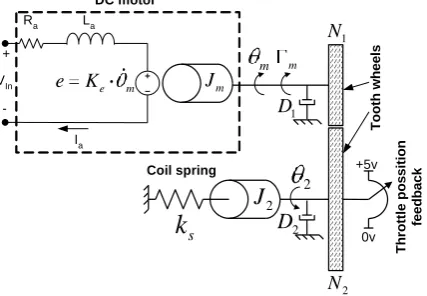
The DC motor drives a gear train that is connected to the throttle plate and a position sensor, as modelled in Figure 2.

La Ra e m e K I_a + -V_In DC motor m m m J 1 D 1 N 2 N 2 D 2 2 J s

k

Figure 2: Throttle system model.

On both sides of the gear there are moments of inertia, J_m and J₂, and kinetic friction (i.e., viscose friction) coefficients, D₁ and

2

D . The DC motor is modelled in the standard form:

a

in a a a e m

di

v t L R i t K t

dt (1)

where i_a, R_a, L_a and K_e are, respectively, the armature current, resistance, inductance and back EMF constant. Rearranging (1):

1 a

in a a e m

a

di

v i R K

dt L (2)

The torque produced by the DC motor is

[ ]

m i ta Kt Nm (3)

where K_t K_e is the motor torque constant. To simplify the model, Jm and D1 are

referred to the right hand side of the gear using 2 2 2 1 m m N N (4)

where N₁ and N₂ are, respectively, the numbers of teeth on the input and output gearwheels. This results in the simplified mechanical subsystem model of Figure 3.

2 1 m N N 2 x D s

k

Figure 3: Simplified mechanical system model

The corresponding torque balance equation is

2 1 2 2 2

m N N Jx Dx ks (5)

where the system inertia and kinetic friction are

2 2

2/ 1 2

x m

J J N N J kg m and

2

1 2 / 1 2 sec/

x

D D N N D Nm rad ,

the coil spring constant is k_s[Nm/rad], the

gear ratio is N₂/N₁ and the DC motor

torque is m[Nm].

Rearranging (5) yields

2

2 2 2

1

1

m x s

x

N

D k

J N (6)

The states for the throttle valve model are chosen as x₁ i_a, x_{2 2} and x_{3 2}. The

measurements are y₁ i_a and y2 2. The state differential equation can be formed from (2), (3) and (6):

1 0 1 1 0

2 2 3 4 2

3 3

. .

0

0

0 1 0 0

in

u

x a a x b

x a a a x V

x x

x = A x + B

where a₀ Ra /La,

1 e 2 / a 1

a K N L N ,

2 t 2 / x 1

a K N J N , a₃ Dx/Jx

4 s / x

a k J and b₀ 1/La.

The measurement equation is

1 1

2 2

3

1 0 0

0 0 1

x y

y C x x

y

x .

(8)

The corresponding block diagram is shown in Figure 4.

2

.

m

.

2

..

2

.

Gear system Gear system

Figure 4: Linear throttle valve model

2.2 Additional nonlinear friction

and hard stop models:

Additional refinements to the model of section 0 are presented here. They are 1) hard stops, 2) initial coil spring torque and 3) a nonlinear friction model.

2.2.1. Hard stops. The throttle plate has a limited range of angles, usually from 0 to about 90°. These mechanical position constrains are called hard stops. These are modelled by applying a restraining torque proportional to the distance by which the angular limits are exceeded, using a relatively large constant of proportionality, as shown in Figure 5.

Figure 5 Hard stop model (MathWorks Inc.)

Hence, when x > H the restraining torque is H x K and when x < L it is x L K.

2.2.2. Initial coil spring torque. The coil spring is pre-stressed in the factory to keep the throttle open in the case of an electrical failure. To model this, a constant torque is added, equal to _{Initial spring} k_s

2.2.3. Nonlinear friction model. Through time, the throttle valve on a vehicle will be exposed to moisture and dirt that infiltrates the mechanical system. This will result in an increase in the friction between relatively moving components.

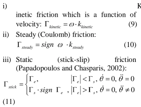
The classical friction model of a bi-directional mechanical system, such as the throttle valve under study, illustrated in Figure 6, comprises three components:

i) K

inetic friction which is a function of velocity: _kinetic k_kinetic (9) ii) Steady (Coulomb) friction:

steady sign ksteady (10)

iii) Static (stick-slip) friction (Papadopoulos and Chasparis, 2002):

, , 0, 0

, , 0, 0

e e s

stick

s sign e e s

(11)

where e is the externally applied torque,

Figure 6: Classic friction model (Papadopoulos and Chasparis, 2002)

This, however, has the drawback of inaccuracy around zero velocity and therefore an improved version will be used. A generic friction model was proposed by (Majd and Simaan, 1995) which includes a more realistic continuous transition between the breakaway torque and the sum of the kinetic and steady torque components of (9) and (10). The nonlinear function used, however, is relatively complicated but the authors have produced a simpler version imposing a lesser computational demand, as follows:

total kinetic steady static yt (12)

where _steady, _kinetic are define by (9) and

(10),

1 1 1

1 ,

1,

t

y (13)

and

static

A

B sign (14)

where A ₁ B ₁ , 1 1 2 2

2 1

B

and ₁ together with ₂ are defined in Figure 7.

total friction

static friction steady friction

kine tic

fric tion

2

2 1 1

Transition section

Figure 7: Friction model and its components.

The following constant parameters are used:

1 0.01 and 2 0.001. 1 kstatic and

2, 2 2 1 were found using the Simulink Parameter Estimation tool.

Finally, Figure 8 shows a simulation of the friction model to be incorporated in the subsequent simulations.

Figure 8: Friction model simulation - _total

3. Throttle valve control:

3.1 Standard PI control

cycling errors that would otherwise be caused by the stick-slip friction component.

Figure 9: Standard PI control loop

3.2 Observer Based Robust Control

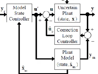
OBRC is a control technique that can be applied to linear and nonlinear plants with disturbances (Dodds, 2007) & (Stadler et al., 2007). Figure 10 shows the general block diagram of this scheme.

Figure 10: OBRC block diagram (Dodds, 2007).

Here, x, y, d and u are, respectively, the plant state, measurement, disturbance and control vectors. This block diagram structure results from the following. First an observer is formed with model state, ˆx_m, and an estimate, ˆu_e, of the disturbance referred to the control input that is equivalent to the combination of d with the theoretical disturbance equivalent to parametric mismatches between the model and the plant. Then ˆu_e is subtracted from both the plant and the model inputs. This converts the problem of controlling the uncertain plant to that of controlling the known model.

Hence the model state controller shown in Figure 10, that responds to the reference input vector, y_r, is designed like any other state space controller. A wide range of plant models is possible with a rank at least equal to that of the real plant but in the system under study, the linear throttle valve model of Figure 4 is used.

Applying the model state control law

2 1ˆ 1 2ˆ 2 3ˆ 3

. r m m m

u r y k x k x k x (15)

where r is the reference input scaling coefficient and k i_i, 1, 2,3 are the state feedback gains, and adding its equivalent block diagram to Figure 4 enables the closed loop transfer function to be derived with the aid of Mason‟s rule, yielding:

1

3 2

1 2 3

r

Y s b

Y s s a s a s a (16)

where: b₁ r k N_{t 2}/ L N J_{a 1 x}

1 a / a x/ x 3/ a

a R L D J k L

2

2 2

2 2

1 1

3

1

1

s t e t

x a x a x

a x x

a x a x

k k k N k N

a k

J L J N L N J

R D D

k

L J L J

2

3 1 3

1

1 1

t a s s

a x a x a x

k N R k k

a k k

L N J L J L J

The Dodds 5% settling time formula (Dodds, 2008) is used to obtain a non overshooting closed loop response with settling time, T_s, by choosing the closed loop characteristic polynomial as

3

3 2

2 3

6 18 108 216

s s s s

s s s s

T T T T (17)

The gains can be found by equating (17) with the denominator of (16).

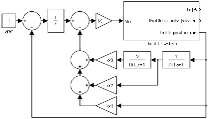
disturbance estimation (referred to the control input), as shown in Figure 11.

2

.

2

..

2

.

ˆ

y

y

u

Figure 11: The observer.

Equating the determinant of Masons rule to zero then yields the observer correction loop characteristic polynomial as follows:

4 3

3 5 1

6 4 2 2 3 5

2

1 3 1 5

3 2 3 6 2 3

1 4 2 1 3 5

4 2

s s q q Ko q q q Ko q q s

Ko q Ko q

Ko q q q Ko q s

Ko q q Ko q q Ko q

(18)

where: q₁ 1/L_a, q₂ k N_{t 2}/ J N_{x 1} , q₃ R_a/L_a,

4 e 2 / a 1

q k N L N , q₅ D_x/J_x and q₆ k_s/J_x Again the Dodds 5% settling time formula is used to design the observer to have a correction loop settling time of T_so:

4 _{4 3 2}

2

3 4

30 1350

15 2

4

13500 50625

8 16

so

so so

so so

s T s s s

T T

s

T T

(19)

Equating (18) and (19) then yields

1 30 / so 3 5

Ko T q q

2

2 6 4 2 3 5

1 3 1 5

1350 / 4 _so

Ko T q q q q q

Ko q Ko q

3

3 6 2 3

3

2

1 4 2 1 3 5

13500 / 8Ts q q Ko q 1

Ko

q

Ko q q Ko q q

4 4

2

50625 1

16 s

Ko

T q

3.3 Sliding Mode Control (SMC):

It is a well documented that sliding mode control (SMC) can achieve robustness in linear and nonlinear systems (Utkin et al., 1999), (Dodds and Vittek, 2009). There are many variations on this theme, some of which are designed to eliminate the control chatter of the basic version. In this investigation, the boundary layer method is employed, equivalent to a high gain output derivative feedback control system. Since the high gain is finite, an outer integral control loop can be added, resulting in the closed loop system of Figure 12.

Figure 12: Boundary layer based SMC with an integrator to remove the steady state error.

The low pass filtering with time constant,

filter

T , is introduced to avoid amplification of

measurement noise at high frequencies.

Again, the Dodds 5% settling time formula is used to determine the three output derivative weights, w1, w2 and w3, assuming the

aforementioned filtering has a negligible effect on the closed loop dynamics, yielding a settling time of T_s as follows:

3

2 3

1 2 2

1 1

1 1

r

Y s

Y s w s w s w s s a (20)

where a Ts/ 6. Then

2 3

1 3 , 2 3 , 3

4. Simulations:

4.1 Parameters:

4.1.1. Throttle valve. The following parameters are found by laboratory tests and the Simulink Parameter Estimation Tool:

0.0261 t

K ; Ke 0.027; Ra 1.25;

0.02 a

L ; J_x 0.003; k_s 0.0932;

2.73

Initial spring ; tsystem delay 0.0011;

8.6119 05

kinetic

k e ; ₂ 0.251;

0.1353 static

k ; ksteady 0.1524.

4.1.2. Conventional PI control loop. The controller gains were adjusted to yield

0.3 s

T s without overshooting: Kp 3.8

and K_I 1.7. The square wave dither amplitude and frequency are, respectively,

1 dither

u V and f_dither 10 Hz .

4.1.3. Observer based robust controller. A settling time of T_s 0.3 s was used to

calculate the state feedback gains: k₁ 1.05, 2 -0.165

k and k₃ -0.047. To maximise the robustness, the minimum observer correction loop settling time was found to be

0.015

so

T . Attempting to reduce this further resulted in undesirable oscillatory behaviour. Observer gains: Ko₁ 1937,

2 1497761

Ko , Ko₃ 4257095 and

4 532141336

Ko .

4.1.4. Sliding mode controller. The output derivative filtering time constant,

0.0005 filt

T , was set to a relatively small

value to avoid limiting the high gain. A settling time T_s 0.3 s was selected to determine the derivative feedback weightings: w₁ 0.15, w₂ 0.0075 and

3 0.000125

w . To maximise the robustness,

the system gain was set to K= 500. Beyond this, the system response became oscillatory.

Step response comparison

In all three Simulink simulations, a stiff numerical integration algorithm was employed to cater for the two robust control techniques. The PI control loop was tuned to achieve a non-overshooting step response with the specified settling time but this entailed much time and effort, in comparison with the SMC and OBRC.

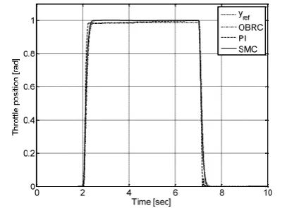
Figure 13 shows the superimposed responses using all three controllers with a reference input commencing at zero, stepping to 1 rad. at t 2 s and returning

to zero at t 7 s .

Since they appear very close together on this amplitude scale, differences in performance are made more visible by plotting the position control errors (Figure 14), defined

as y t yideal t , where yideal t is the step

response that the system is designed to achieve ideally.

Figure 14: Step response errors

It is evident that the PI control yielded the worst errors. As expected the robust control methods yielded better responses but the SMC has a smaller error than the OBRC.

4.2

Ramp

response

control

comparison

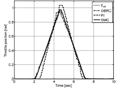
Since the throttle position demand is continuous during the normal operation of an engine management system, the second reference input used for performance comparisons ramps up at 1 rad s/ from

zero at t 2 s and at t 5 s ramps down at

1 rad s/ to zero at t 7 s , remaining zero thereafter. The results are shown in Figures 15 and 16.

Figure 15: Ramp responses.

Figure 16: Ramp response errors.

Despite the control dither, the PI control loop is adversely affected by the stick-slip friction. As for the step responses, both the robust controllers improve on this but the SMC performs better than the OBRC.

5.

Conclusions

and

Recommendations:

It is remarkable that even without control dither, the robust controllers performed better that the PI controller with the control dither. Furthermore, it is recommended that a fairer comparison be carried out by applying control dither with all three controllers.

The different plant models such as the multiple integrators (Dodds, 2007) should be considered in case this permits a smaller value of T_so and therefore higher robustness. Finally, experimental work currently in progress will be published later.

6. References

DODDS, S. J. (2007) Observer based robust control. AC&T.

DODDS, S. J. (2008) Settling time formulae for the design of control systems with linear closed loop dynamics. AC&T.

DODDS, S. J. & VITTEK, J. (2009) Sliding mode vector control of PMSM drives with flexible couplings in motion control. AC&T. MAJD, V. J. & SIMAAN, M. A. (1995) A continuous friction model for servo systems with stiction. Proceedings of the 4th IEEE Conference on Control Applications.

PAPADOPOULOS, E. G. & CHASPARIS, G. C. (2002) Analysis and model-based

control of servomechanisms with friction. IEEE/RSJ International Conference on Intelligent Robots and Systems.

STADLER, P. A., DODDS, S. J. & WILD, H. G. (2007) Observer based robust control of a linear motor actuated vacuum air bearing. AC&T.