Performance Evaluation of the Cognitive Packet
Network in the Presence of Network Worms
GEORGIA SAKELLARI
Imperial College London,,Intelligent Systems and Networks Group Electrical & Electronic Engineering Dept., Imperial College, London SW7 2BT.
Abstract
Reliable networks that provide good service quality are expected to become more crucial in every aspect of communication, especially as the information transferred between network users gets more complex and demanding and as malicious users try to deliberately degrade or altogether deny legitimate network service. The Cognitive Packet Network (CPN) routing protocol pro-vides Quality of Service (QoS) driven routing and performs self-improvement in a distributed manner, by learning from the experience of special packets, which gather on-line QoS measurements and discover new routes. Although CPN is generally very resilient to network changes, it may suffer worse per-formance during node failures caused by network threats, such as network worms. Here we evaluate the performance of CPN in such crises and compare it with the Open Shortest Path First (OSPF) routing protocol, an industry standard and widely used in Internet Protocol networks. We also improve it by introducing a failure detection element that reduces packet loss and delay during failures. Our experiments were performed in a real networking testbed.
Key words:
1. Introduction
their destination and proposes randomised routing policies which can improve QoS. The Cognitive Packet Network (CPN) is a QoS-based routing proto-col and has been shown to adapt quickly to varying network conditions and user requirements [21]. Contrary to conventional mechanisms, it is the users rather than the nodes that control the routing, by specifying their desired QoS criteria and the network tries to route each one of them individually based on his/her needs. CPN was also proposed for ad hoc networks which provides dynamic discovery of paths that offer both low-delay and energy efficiency [13]. CPN has been evaluated extensively under normal operating conditions and has proven to be very adaptive to network changes such as congestion. Here we investigate the performance of CPN under catastrophic node failures caused by the spread of network worms.
The paper is organised as follows: Section 2 provides a brief overview of the CPN routing protocol. In Section 3, we present previous work evaluating the performance of CPN. In Section 4, we introduce a failure detection ele-ment in the CPN mechanism which improves its performance. In Section 5 we present experiments we conducted specifically for network node failures propagated as network worms and generated by a failure emulator of our design. We conclude in Section 6 with a summary of our contributions and suggested future work.
2. Overview of CPN
CPN is an adaptive packet routing protocol that addresses QoS by using adaptive techniques based on on-line measurements [14, 17, 15, 12, 7, 27]. It is a distributed protocol with which users, or the network itself, declare their QoS Goals, such as minimum Delay, maximum Bandwidth, minimum Packet Loss, minimum Variance of the packet delay, maximum Security Level in a path, minimum Power Consumption in a wireless node, or a weighted combination of these. It is designed to perform self-improvement by learning from the experience of special packets that constantly probe the network.
More specifically, it makes use of three types of packets; smart packets (SP) for discovery, source routed dumb packets (DP) to carry the payload and acknowledgement (ACK) packets to bring back information that has been discovered by SPs, and is used in nodes to train neural networks and produce routing decisions. The role of SPs is to explore the network and discover the best routes, according to a QoS goal, for each source-destination pair in the network. At each hop SPs are routed according to the experiences
of previous packets with the same goals and the same destination. The term “goal” is used instead of “QoS specifications” to emphasize the fact that there are no QoS guarantees and that CPN provides a best effort service [30]. The decisions of the SPs are based on a learning algorithm. In order to explore all possible routes, at some hops, each SP makes a random routing decision, with a small probability (usually 5%). To avoid overburdening the system with unsuccessful requests or packets which are in effect lost, all packets have a life-time constraint based on the number of nodes they have visited.
Several algorithms have been used in CPN as learning and decision tech-niques in order for SPs to find satisfactory routes from source to destination based on the desired goals. As far as the decision process is concerned, Ran-dom Neural Networks (RNNs) [5] are mainly used. The RNN is a biologically inspired neural network model which is characterised by the existence of posi-tive (excitation) and negaposi-tive (inhibition) signals in the form of spikes of unit amplitude that circulate among nodes and alter the potential of the neurons. Each neuron can be connected to another neuron and each connection is char-acterized by an excitatory or inhibitory weight [20]. The state of a neuron, which represents the probability that the neuron is excited, has been proven to satisfy a system of nonlinear equations with a unique solution. Therefore, in a CPN network, at each node a specific RNN that has as many neurons as the possible outgoing links, could represent the decision to choose a given output link for a smart packet. The arrival of SPs triggers the execution of RNN and the routing decision is the output link corresponding to the most excited neuron.
As far as the learning process used with RNN, the algorithm that even-tually prevailed in the implementations of CPN is Reinforcement Learning (RL). RL is used to change neuron weights in order to reward or punish a neuron according to the level of goal satisfaction measured on the corre-sponding output. Therefore the decisional weights of a RNN are increased or decreased based on the observed success or failure of subsequent SPs to achieve the goal. Thus RL will tend to prefer better routing schemes, more reliable access paths and better QoS.
3. Previous Work on Performance Evaluation of CPN
ex-perimental work conducted in the past in order to evaluate the performance of CPN. All performance evaluation work has been carried out in a real networking testbed, running CPN as a module of the Linux kernel.
3.1. Adaptability
CPN’s ability to adapt to changing network conditions, such as changes in traffic load, link failures, or buffer overflows has been experimentally eval-uated in [18]. The experiments showed that CPN managed to find new routes in order to avoid obstructing traffic that was introduced in some of the links used by the data traffic and also avoided links that where under failures. Another issue studied experimentally in [18] was the effect of the ratio of SPs on overall performance, which was was further investigated in [16]. The experiments concluded that in order to achieve the best performance for the data packets (DPs) the percentage of SPs that should be sent for discovery is 10% to 20% of the data packets’ rate. Going beyond these values does not significantly improve the QoS values for DPs. One must bear in mind that in CPN, SPs and ACKs are not full sized Ethernet packets, but are actually 10% of the DPs’ size. If 20% of SP traffic is added, this will result in 14% traffic overhead, when ACKs are generated by both DPs and SPs, and only 4% of traffic overhead when ACKs are only generated in response to SPs. Additionally it was shown that a small number of SPs can suffice to initially establish a connection.
3.2. QoS Goals
The experiments in [19] show that CPN can implement distributed adap-tive shortest-path routing and approximately find shortest paths. Extensive experiments compare the shortest-path CPN, where the QoS goal is the min-imum hop count, with a CPN routing using minmin-imum-delay and a version where routing is based on a combination of hop count and forward delay. The experiments, conducted under low, medium and high background traf-fic, show that the use of criteria more complex than the shortest number of hops, can provide better overall quality of service.
The choice of a “goal” and “reward” function for packetised voice ap-plications is discussed in [15], where experiments conducted for ”voice over CPN” are presented. The performance of CPN is detailed via several mea-surements showing that the resulting QoS is better than when using IP in identical conditions. Measurements indicating how the CPN protocol can respond to different QoS goals are also presented in [12, 30]. Composite goal
functions which take into account both delay and packet loss are proposed. In [30], the measurements suggest that CPN networks effectively adapt routing behaviour to the QoS goal that is specified.
The use of delay as a QoS goal implies the collection of timestamps along packets paths, which add overhead to the packets, especially in long paths. Therefore, the authors of [24] have implemented a composite QoS goal metric which consists of path length and buffer occupancy of nodes to achieve traffic balancing and to identify low-delay paths in a network. Experimental results in a wired testbed and wireless ad hoc simulations show that a routing goal that combines path length and buffer occupancy in nodes offers the advantage of producing approximately the same performance as that of using delay, but with less packet overhead.
3.3. Routing Oscillations
Although oscillations are generally considered as a weakness of a net-work, performance evaluations in [22] indicate that routing oscillations do not severely degrade performance as would be expected, and high perfor-mance can still be obtained. The authors of [22, 11] study the way that oscillations can be controlled. Two different parameters that affect oscilla-tions are considered: the use of probabilistic path switching, which can be used both to make path switching more asynchronous and to vary the rate at which switching decisions are made, and the introduction of a decision threshold which will only allow path switching if the gain expected from switching exceeds a certain minimal value. Both of these control schemes are easy to implement and provide an effective way to limit oscillations and their negative consequences.
3.4. Realistic environments
the cost of each link is proportional to its delay, OSPF routing converges to the minimal delay path, giving a baseline for comparison. The experi-ments show that the routes CPN computes are as good as those computed a priori using administrator-defined costs. Furthermore, the paper gives exper-imental results showing that RNN with RL can autonomously learn the best route in the network simply through exploration in a very short time-frame and demonstrates that the CPN protocol is able to adapt to changes in the network environment quickly, by switching to a new optimal route in the network.
4. Enhancing the Failure-Awareness of CPN
Currently, each CPN node detects failures by sending “hello” messages to its neighbours. This way a neuron (link) is excluded from a decision only if one of a node’s neighbours is under failure. Thus, CPN does not take into consideration failures which could be further away and can influence the selection of a specific link. Additionally, the weights of the RNNs in a node are updated only when an ACK packet returns to it. Therefore, if a node which is part of a selected route suffers a failure, the ACKs returning to the source through that same route will never reach the source and the weights of the neurons corresponding to the links that are affected by the failure will never be punished. To prevent this, CPN nodes route a fraction of the SPs randomly, so that sudden changes of any kind could be discovered. But even with this technique, in some failure scenarios it may need considerable numbers of random SPs before the decision of a node changes. For example, if the neuron which corresponds to the node/path under failure was previously chosen a lot of times, and thus has a much higher weight than the rest of the neurons, it might need a big number of random SPs to discover another path. Thus, if that neuron was the most excited, the subsequent source-routed data packets will continue to follow the path under failure and will be lost until a new path is discovered. In this section we propose a detection mechanism that makes the neurons of CPN more failure-aware.
In our scheme, which was first introduced in [28], a neuron can be consid-ered under failure even if the first hop neighbour node is not under failure, because it may be part of a path that has failed. More specifically, at each
RNN and for each neuron i, the timestamp of the last SP and the last ACK
that used it, are stored. If no ACK has been received after sending the last SP:
timestamp of last SP going through i−ε < timestamp of last ACK coming through i (1)
then the link is considered “under failure” and the neuron corresponding to this link is considered “expired”. Expired neurons do not participate in the calculation of the excitatory probabilities and the subsequent decisions
of the RNN. The value ofεmay be different for each neuron and may depend
on the average delay between the node and the destination, under normal conditions. The neuron is just ignored and its weights do not change so that they can be used again either after the failure restoration or if another path is discovered that bypasses the failure.
5. Performance evaluation of CPN under node failures propagating as a network worm
5.1. Network worms
Network worms are malicious self-replicating and self-propagating appli-cations that exploit system vulnerabilities of some operating systems and spread through networks. Their defining characteristic is their ability to achieve high infection rates; they can spread and saturate a network very quickly. The results of such attacks could be mild, such as the printout of a message or more serious such as deleting or modifying system files, reducing the system performance, or causing total failure to the infected machines. From the service quality perspective and according to the extent of the spread, the latter could lead to serious agitation for the users of the network, due to information loss and delays.
Network worms use a number of different methods to identify new targets for infection; for example, many worms scan randomly generated IP addresses to locate vulnerable hosts (random scan), or scan the IP address space based on the route information in a network (routable scan), or acquire a target address table from the DNS server (DNS scan), or create a pre-generated tar-get list which includes vulnerable hosts and then try to infect the computers listed there (hit-list scan) [29, 26, 32]
a virus, the host remains in the infectious state forever [26, 2]. Unlike the SEM model, in the Kermack-Mckendrick (KM) model the host maintains one of three states: susceptible, infectious or removed [26, 4]. When an infected host is immunised it is removed from the whole system and does not take into consideration situations where susceptible and infected hosts are patched to resist the worm. The Susceptible-Infectious-Susceptible (SIS) model assumes every host has the same possibility of being infected repeatedly even if they have recovered but does not take into account the situation that the infected hosts are patched or updated to be immune from the worms [26, 1].
The Two-Factor model is the extension and supplement of SEM and KM and considers more external factors and anti-worm measures [26, 31]. One factor is the dynamic countermeasures taken by ISPs and users and the other is the slowed down worm infection rate because rampant propagation of worm causes congestion and troubles to some routers. It does not consider though the patching of the infected hosts. The Worm-Anti-Worm model takes into account the existence of an antagonistic worm and considers two types of worms, the malicious worm and an oppositional one, which can detect, clean and patch the hosts infected by the malicious worms[26]. It does not consider though the states of the antagonistic worm after it enters the susceptible hosts.
The patching effect and the ability to resist specific worms while being susceptive to others is addressed in [8, 9]. The author, inspired by biological viruses, proposes a probability model for populations of agents (computer software) and viruses (computer worms) that interact in the presence of an anti-viral agent. Both agents and viruses can belong to different strains. If a virus survives the effect of the anti-viral agent it belongs to a different strain from the one it started in, and its ability to survive future encounters or infect healthy agents is modified. Similarly, an agent which remains healthy after an encounter with a virus will belong to a new strain and this will impact its future behaviour. Also, an antiviral agent can be made up of a mix or cocktail, with different proportions of agents that target different strains of the virus.
In our experiments, the failures are spread according to the Analytical Active Worm Propagation (AAWP) model. This is a discrete-time and con-tinuous state deterministic approximation model, proposed by Chen et al. to model the spread of active worms that employ random scanning [3]. In the AAWP model, a node can be in one of the following states: infected, immunised, vulnerable. In our present application we have assumed that
all hosts can reach (infect or immunise) each other directly (the topology of the network is irrelevant). At each scan, the “worm” randomly chooses another host of the population and if it is immune nothing happens. If it is vulnerable it becomes infected and if it is already infected, it does not get re-infected. We assume that the infection delay time between two consecutive infection attempts represents the time required by a computer worm to find a server through random IP scans, regardless of whether the host is already infected or still vulnerable. So, a computer cannot infect other hosts before it is infected completely. In our implementation, the time the worm needs to infect a machine, called the infection delay time, is a random value within a predetermined range, but the emulator could be extended so that the infec-tion delay time could be subtracted by a more complex model which takes into account the distance between the infected node and the node it tries to infect, the degree of network congestion and other such parameters. When a node is infected it is considered under failure but it can still infect others. Finally, in order to capture the patching impact on the worm propagation, we dynamically immunise some hosts, which, after some time, start immunising others (infected or simply vulnerable) randomly. The time a newly immu-nised node has to wait before it starts immunising others is again a random value. The scanning mechanism used is the random scanning mechanism but others could be used, such as local subnet and topological scanning.
5.2. Failure Emulator
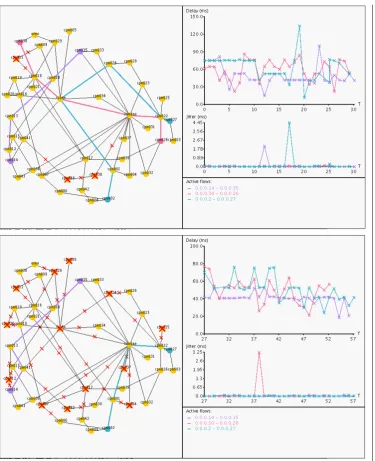
Figure 1: Snapshots of the failure emulator at the beginning of the failure spread and after the failures have spread throughout the network.
5.3. Configuration of the experiments
The experiments were conducted on a 46 node testbed (figure 2). The
topology of the testbed represents the real SWITCHlan network topology1.
1The Swiss Education & Research Network (SWITCHlan) network provides service in Switzerland to all universities, two federal institutes of technology and major research
In order to make the environment more realistic we used actual details of the 46-router backbone, complete with bandwidth, OSPF costs, and link-level delays which were given by the administrators of the SwitchLAN network to the authors of [23]. We have also configured IP routing using quagga 0.99.3 with the OSPF costs of the SwitchLAN network so that the routes in our testbed should be exactly the same as those used in the real Swiss backbone. Because the cost of each link is proportional to its delay, OSPF routing converges to the minimal delay path, giving a baseline for comparison.
Figure 2: Realistic topology with artificial delays. The thickness of the links represents their delay. The grey and thinner lines are low-delay links, while the darker (blacker) and thicker ones denote higher delays
There are three Source-Destination (S-D) pairs that correspond to three
users in the network. Each user generates UDP traffic at constant bitrate of 6M bps. At the beginning of the experiment all nodes are vulnerable except the sources and destinations. All the sources and destinations are immune so
that they will not suffer a failure. Each experiment lasts for 120s. The failure
propagation starts 10safter the start the experiment and its duration varies
according to the scanning rate. The higher the scanning rate the more the number of infected nodes, and therefore the longer the network will operate in difficult conditions and experience congestion. More analytically:
• The number of machines that are already infected at the start of the
“worm’s” propagation is 1.
• The scanning rate varies within the range [0.05, 0.1, 0.2, 0.3, 0.4, 0.5,
0.6, 0.7] scans/s, which corresponds to 1 node being scanned every [10, 5, 3.33, 2.5, 2, 1.67, 1.43] s respectively.
• The duration of the experiment is 120s.
• The worm propagation starts at the 10th second.
• A newly infected node has to wait for a given delay before it starts
in-fecting others. In our experiments that delay is a random value between 15 and 20s.
• When a node is infected it is considered to be under failure, traffic
cannot go though it (Ethernet interfaces are disabled) but it can still infect others.
• The patching process starts at the 70th second (60s after the start of
the failure propagation) and the patching rate is equal to 0.5 node/s.
Finally, before it starts immunising others, a newly immunised node has to wait a random value between 15 and 20s.
5.4. Experimental results
In the figures presented next we compare the performance of CPN to that of OSPF routing protocol and to our proposed failure-aware CPN. Each experiment was conducted 10 times and the values presented are the average of these runs. The values missing in the delay graphs are due to the fact that at those points, most of the network nodes were under failure and there was no route connecting at least one user’s source and destination. This is also
confirmed by the loss graphs since at those points the packet loss is equal to 100%. Having 100% packet loss in some cases is not unrealistic. It is due to the fact that we have a relatively small testbed and the effects of the failure spread in such a network lead to the saturation of the network by the failures and thus it is very probable that there is no path between the source and the destination of a user, which in turn leads to total loss of the data packets.
0 20 40 60 80 100 120
0 10 20 30 40 50 60 70 80 90 100
Average Packet Loss, Scanning rate = 0.05
Time (s)
Average Packet Loss (%)
IP Current CPN Failure−Aware CPN
0 20 40 60 80 100 120
0 50 100 150 200 250 300 350
Average Delay, Scanning rate = 0.05
Time (s)
Average Delay (ms)
[image:13.595.120.489.231.378.2]IP Current CPN Failure−Aware CPN
Figure 3: Average Packet Loss and Average Delay for all 3 users when scanning rate = 0.05 nodes/s
0 20 40 60 80 100 120
0 10 20 30 40 50 60 70 80 90 100
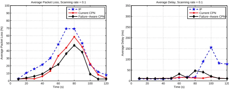
Average Packet Loss, Scanning rate = 0.1
Time (s)
Average Packet Loss (%)
IP Current CPN Failure−Aware CPN
0 20 40 60 80 100 120
0 50 100 150 200 250 300 350
Average Delay, Scanning rate = 0.1
Time (s)
Average Delay (ms)
IP Current CPN Failure−Aware CPN
[image:13.595.120.488.440.585.2]0 20 40 60 80 100 120 0 10 20 30 40 50 60 70 80 90 100
Average Packet Loss, Scanning rate = 0.2
Time (s)
Average Packet Loss (%)
IP Current CPN Failure−Aware CPN
0 20 40 60 80 100 120
0 50 100 150 200 250 300 350
Average Delay, Scanning rate = 0.2
Time (s)
Average Delay (ms)
[image:14.595.121.486.129.275.2]IP Current CPN Failure−Aware CPN
Figure 5: Average Packet Loss and Average Delay for all 3 users when scanning rate = 0.2 nodes/s
0 20 40 60 80 100 120
0 10 20 30 40 50 60 70 80 90 100
Average Packet Loss, Scanning rate = 0.3
Time (s)
Average Packet Loss (%)
IP Current CPN Failure−Aware CPN
0 20 40 60 80 100 120
0 50 100 150 200 250 300 350
Average Delay, Scanning rate = 0.3
Time (s)
Average Delay (ms)
[image:14.595.120.488.323.470.2]IP Current CPN Failure−Aware CPN
Figure 6: Average Packet Loss and Average Delay for all 3 users when scanning rate = 0.3 nodes/s
0 20 40 60 80 100 120
0 10 20 30 40 50 60 70 80 90 100
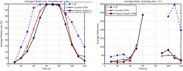
Average Packet Loss, Scanning rate = 0.4
Time (s)
Average Packet Loss (%)
IP Current CPN Failure−Aware CPN
0 20 40 60 80 100 120
0 50 100 150 200 250 300 350
Average Delay, Scanning rate = 0.4
Time (s)
Average Delay (ms)
IP Current CPN Failure−Aware CPN
Figure 7: Average Packet Loss and Average Delay for all 3 users when scanning rate = 0.4 nodes/s
[image:14.595.120.489.519.663.2]0 20 40 60 80 100 120 0 10 20 30 40 50 60 70 80 90 100
Average Packet Loss, Scanning rate = 0.5
Time (s)
Average Packet Loss (%)
IP Current CPN Failure−Aware CPN
0 20 40 60 80 100 120
0 50 100 150 200 250 300 350
Average Delay, Scanning rate = 0.5
Time (s)
Average Delay (ms)
[image:15.595.120.489.129.275.2]IP Current CPN Failure−Aware CPN
Figure 8: Average Packet Loss and Average Delay for all 3 users when scanning rate = 0.5 nodes/s
0 20 40 60 80 100 120
0 10 20 30 40 50 60 70 80 90 100
Average Packet Loss, Scanning rate = 0.6
Time (s)
Average Packet Loss (%)
IP Current CPN Failure−Aware CPN
0 20 40 60 80 100 120
0 50 100 150 200 250 300 350
Average Delay, Scanning rate = 0.6
Time (s)
Average Delay (ms)
[image:15.595.120.489.323.470.2]IP Current CPN Failure−Aware CPN
Figure 9: Average Packet Loss and Average Delay for all 3 users when scanning rate = 0.6 nodes/s
0 20 40 60 80 100 120
0 10 20 30 40 50 60 70 80 90 100
Average Packet Loss, Scanning rate = 0.7
Time (s)
Average Packet Loss (%)
IP Current CPN Failure−Aware CPN
0 20 40 60 80 100 120
0 50 100 150 200 250 300 350
Average Delay, Scanning rate = 0.7
Time (s)
Average Delay (ms)
IP Current CPN Failure−Aware CPN
[image:15.595.119.490.519.663.2]Figures 3-10 show the average packet loss and delay of all three users throughout the duration of the experiment.It is evident that by using CPN we have significantly less packet losses than when using OSPF. Also, packet losses are further reduced when we use the failure-aware version of CPN. The fact that with CPN and especially with the failure-aware CPN the network has reached 100% losses less times, means that it had detected and avoided the failures more quickly and had found paths between the sources and the destinations when OSPF could not. As far as the delay is concerned, both versions of CPN have kept the delay values lower than the OSPF. The failure-aware CPN manages to keep the delay values in the same levels, if not better, with the current CPN. In all cases the CPN protocol, on average, performs better than OSPF and our failure-aware CPN has generally improved the performance of CPN in respect to packet loss and has kept delay in the same levels. This is more obvious in the summarised results presented next.
5.4.1. Result summary
Below we summarise the previous results of all the scanning rates into one figure for the average packet loss and one figure for the average delay for all users in the network.
0 0.1 0.2 0.3 0.4 0.5 0.6 0.7 0
10 20 30 40 50 60 70 80 90 100
Total Packet Loss
Scanning Rate (nodes/s)
Packet Loss (%)
IP Current CPN Failure−Aware CPN
0 0.1 0.2 0.3 0.4 0.5 0.6 0.7 0
50 100 150 200 250
Total Delay
Scanning Rate (nodes/s)
Delay (ms)
[image:16.595.121.502.414.566.2]IP Current CPN Failure−Aware CPN
Figure 11: Average Packet Loss and Average Delay for all users when scanning rate = [0.05 0.1, 0.2, 0.3, 0.4, 0.5, 0.6, 0.7] nodes/s
Figure 11 presents the average packet loss and delay for all three users. As expected the average packet loss increases as the scanning rate increases since the infected nodes increase. The results show that, on average, the QoS of the users is significantly improved when using the failure-aware CPN.
Users lose less data during the experiment while the delay is kept on more or less the same levels. This means that failure-aware CPN has detected and avoided the failures more quickly than both the current CPN and OSPF.
6. Conclusions
In this paper we evaluated the performance of the CPN routing protocol in the presence of network worms which cause node failures. We provided experimental results showing the resilience of CPN and its comparison with the IP protocol. The experiments were conducted in a real testbed and the results demonstrate CPN’s ability to guide the network during a crisis by adapting quickly to the network changes without significantly affecting the QoS provided to the users of the network. We have also described a failure detection element which is shown to further improve the performance of CPN during failures.
Further work could include experimental evaluations in scenarios of worm propagations based on epidemiological models or mathematical models de-rived from empirical data. Also, we acknowledge that we conducted the experiments in a testbed that is relatively small in the context of epidemics. In order to investigate epidemics we need a significantly larger network by using for example PlanetLab nodes [25]. Furthermore, the failure detection component proposed in section 4 could be further improved by finding the optimal time a node has to wait until it considers a link part of a failed path. Finally, the failure emulator described in section 5.2 can be used to identify the real-time network parameters that could proclaim the existence of a computer worm before it actually spreads throughout the network.
References
[1] Allen, L., Burgin, A., Jan. 2000. Comparison of deterministic and stochastic SIS and SIR models in discrete time. Mathematical Bio-sciences 163 (1), 1–33.
[2] Andersson, H., Britton, T., 2000. Stochastic Epidemic Models and Their Statistical Analysis. Springer-Verlag, New York.
[4] Frauenthal, J., 1980. Mathematical modeling in epidemiology. Springer-Verlag, New York.
[5] Gelenbe, E., 1989. Random Neural Networks with Negative and Positive Signals and Product Form Solution. Neural computation 1 (4), 502–510.
[6] Gelenbe, E., Dec. 2003. Sensible decisions based on QoS. Computational Management Science 1 (1), 1–14.
[7] Gelenbe, E., Oct. 2004. Cognitive Packet Network. US Patent 6804201 B1.
[8] Gelenbe, E., Oct. 2005. Keeping Viruses Under Control. In: Proceed-ings of the 20th International Symposium on Computer and Information Sciences(ISCIS 2005), Lecture Notes in Computer Science, Vol. 3733. Springer Verlag, New York and Berlin, Istanbul, Turkey, pp. 1–1.
[9] Gelenbe, E., Sep. 2007. Dealing with software viruses: a biological paradigm. Information Security Technical Reports 12 (4), 242–250.
[10] Gelenbe, E., July 2009. Steps toward self-aware networks. Communica-tions of the ACM 52 (7), 66–75.
[11] Gelenbe, E., Gellman, M., Oct. 2007. Oscillations in a Bio-Inspired Routing Algorithm. In: Proceeding of the IEEE Internatonal Conference on Mobile Adhoc and Sensor Systems (MASS 2007), BIONETWORKS Workshop. Pisa, Italy, pp. 1–7.
[12] Gelenbe, E., Gellman, M., Lent, R., Liu, P., Su, P., May 2004. Au-tonomous Smart Routing for Network QoS. In: Proceedings of the First International Conference on Autonomic Computing (ICAC). New York, NY, USA, pp. 232–239.
[13] Gelenbe, E., Lent, R., July 2004. Power-aware ad hoc cognitive packet networks. Ad Hoc Networks Journal 2 (3), 205–216.
[14] Gelenbe, E., Lent, R., Montuori, A., Xu, Z., Aug. 2000. Towards Net-works with Cognitive Packets. In: Proceedings of the 8th International Symposium on Modeling, Analysis and Simulation of Computer and Telecommunication Systems (IEEE MASCOTS). San Francisco, CA, USA, pp. 3–12, opening Invited Paper.
[15] Gelenbe, E., Lent, R., Montuori, A., Xu, Z., Oct. 2002. Cognitive Packet Networks: QoS and Performance. In: Proceedings of the 10th IEEE In-ternational Symposium on Modeling, Analysis, and Simulation of Com-puter and Telecommunications Systems (MASCOTS’02). Fort Worth, Texas, USA, pp. 3–9, opening Keynote Paper.
[16] Gelenbe, E., Lent, R., Nunez, A., Sep. 2004. Self-Aware Networks and QoS. Proceedings of the IEEE 92 (9), 1478–1489.
[17] Gelenbe, E., Lent, R., Xu, Z., Oct. 2001. Design and Performance of Cognitive Packet Networks. Performance Evaluation 46 (2-3), 155–176.
[18] Gelenbe, E., Lent, R., Xu, Z., Dec. 2001. Measurement and Performance of a Cognitive Packet Network. Computer Networks 37 (6), 691–701.
[19] Gelenbe, E., Liu, P., June 2005. QoS and Routing in the Cognitive Packet Network. In: Proceedings of First International IEEE WoWMoM Workshop on Autonomic Communications and Computing (ACC’05). Taormina, Italy, pp. 517–521.
[20] Gelenbe, E., Seref, E., Xu, Z., Feb. 2001. Simulation with Learning Agents. Proceedings of the IEEE 89 (2), 148–157.
[21] Gelenbe, E., Xu, Z., Seref, E., Nov. 1999. Cognitive Packet Networks. In: Proceedings of the 11th International Conference on Tools with Artificial Intelligence (ICTAI ’99). IEEE Computer Society Press, Chicago, IL, USA, pp. 47–54.
[22] Gellman, M., Aug. 2008. Oscillations in Self-Aware Networks. Proceed-ings of the Royal Society 464 (2096), 2169–2185.
[23] Gellman, M., Liu, P., Sep. 2006. Random Neural Networks for the Adap-tive Control of Packet Networks. In: Proceedings of the 16th Interna-tional Conference on Artificial Neural Networks (ICANN 2006). Athens, Greece, pp. 313–320.
[25] Paterson, L., Roscoe, T., June 2004. The Design Principles of PlanetLab. Tech. rep., Technical Report PDN04021, PlanetLab Consortium.
[26] Qing, S., Wen, W., June 2005. A survey and trends on Internet worms. Computers & Security 24 (4), 334–346.
[27] Sakellari, G., June 2009. The Cognitive Packet Network: A Survey. The Computer Journal: Special Issue on Random Neural Networks, doi:10.1093/comjnl/bxp053 53 (3), 268–279.
[28] Sakellari, G., Gelenbe, E., May 2009. Adaptive Resilience of the Cogni-tive Packet Network in the presence of Network Worms. In: Proceedings of the NATO Symposium on C3I for Crisis, Emergency and Consequence Management. Bucharest, Romania, pp. 16:1–16:14.
[29] Staniford, S., Paxson, V., Weaver, N., Aug. 2002. How to 0wn the Inter-net in Your Spare Time. In: Proceedings of the 11th USENIX Security Symposium (Security ’02). San Francisco, CA, USA, pp. 149–167.
[30] Su, P., Gellman, M., June 2004. Using adaptive routing to achieve Qual-ity of Service. Performance Evaluation 57 (2), 105–119.
[31] Zou, C., Gong, W., Towsley, D., Nov. 2002. Code Red Worm Propaga-tion Modeling and Analysis. In: Proceedings of the 9th ACM conference on Computer and Communications Security (CCS’02). Washington, DC, USA, pp. 138–147.
[32] Zou, C., Towsley, D., Gong, W., July 2006. On the performance of internet worm scanning strategies. Performance Evaluation 63 (7), 700– 723.


![Figure 11: Average Packet Loss and Average Delay for all users when scanning rate =[0.05 0.1, 0.2, 0.3, 0.4, 0.5, 0.6, 0.7] nodes/s](https://thumb-us.123doks.com/thumbv2/123dok_us/446059.1044126/16.595.121.502.414.566/figure-average-packet-loss-average-delay-users-scanning.webp)
