An exploratory study of GPS trajectory data using Snap Drift Neural Network

Author(s): Ekpenyong, Frank; Palmer-Brown, Dominic; Brimicombe, Allan

Title:An exploratory study of GPS trajectory data using Snap-Drift Neural Network

Year of publication: 2008

Citation: Ekpenyong, F., Palmer-Brown, D., Brimicombe, A. (2008) ‘An exploratory study of GPS trajectory data using Snap-Drift Neural Network’ Proceedings of Advances in Computing and Technology, (AC&T) The School of Computing and Technology 3rd Annual Conference, University of East London, pp.22-30

Link to published version:

An exploratory study of GPS trajectory data using Snap-Drift

Neural Network

Frank Ekpenyong

, Dominic Palmer-Brown

, Allan Brimicombe

Email :{[email protected], [email protected], [email protected]}

Abstract: Research towards an innovative solution to the problem of automated updating of road network

databases is presented. It moves away from existing methods where vendors of road network databases either go through the time consuming and logistically challenging process of driving along roads to register changes or use update methods that rely on remote sensing images. For this approach we hypothesize that users of road network dependent applications (e.g. in-car navigation system or NavSat) could passively record drive trajectories with the on-board GPS, which would inform digital road network data providers if the user was on a road that departs from the known roads in the database. Then such drive characteristics would be collected using the on-board GPS on behalf of the provider. These data would be processed either by an on-board artificial neural network (ANN) or transferred back to the NavSat provider and input to an ANN along with similar track data provided by other service users, to decide whether or not to automatically update (add) the “unknown road” to the road database. As part of this work, in this paper we carry out an exploratory study on the trajectory information recorded with GPS. Trajectory data collected in London are analysed using a Snap-Drift Neural Network (SDNN) which categorises them into their strongest natural groupings, by combining clustering with feature detection in a single ANN. We investigate how the SDNN groups spatio-temporal variations associated with road traffic conditions. These variations are present in the recorded GPS trajectory data. For our approach which relies on users to passively record drive trajectory which are then processed as roads or not roads (Ekpenyong et al., 2007a), it is important to investigate how these variations affects the recorded GPS which influences the grouping by the SDNN. For our approach a question like – how would SDNN groups GPS recorded on a road segment in the morning (supposedly heavy traffic) to that recorded in the day (less traffic)? This issue is investigated in this paper.

1. Introduction

Keeping the road network database up-to-date is important to many Geographic Information System (GIS) applications. Various existing and emerging applications require in particular up-to-date, accurate and sufficiently detailed road databases. Examples are in-car navigation, tourism, traffic and fleet management and monitoring, intelligent transportation systems, internet-based map services, and location-based services (Zhang, 2004a). Due to increasing traffic density, automatic navigation systems for cars and trucks are gaining in popularity (Holzapfel et al.,

uses the trajectory of moving vehicles to automate the detection of new roads and thus update a road network database. It is envisaged that users of in-car navigation system or NavSat would passively collect characteristics of any “unknown route” (departure from the known roads in the database) using the on-board GPS. These data would then be processed either by an on-board neural network or transferred back to the NavSat provider and input to a neural net (ANN) along with similar track data provided by other service users In this approach, Artificial Neural Network (ANN) is used to group the recorded trajectories

patterns found by the SDNN match classes of road and other road network related features. Earlier studies with simulated and real trajectory data informed that the Snap-Drift Neural Network (SDNN) offers a fast method of learning that preserves feature discovery and is capable of grouping moving object characteristics according to their local context information. In most cases the group road features correspond to the travelled road class (Ekpenyong et al., 2007b). For this study, we investigate how the SDNN deals (group) with spatio-temporal variations associated with road traffic conditions.

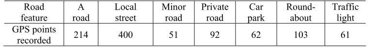
Road

feature road A Local street Minor road Private road park Car Round-about Traffic light GPS points

recorded 214 400 51 92 62 103 61

Table 1: composition of the GPS-based trajectory data within the different road features

2. Raw data

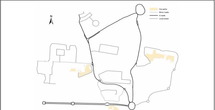
GPS based trajectory data was gathered from a 31.2 km drive over a range of road types in London (Figure 1). The points were recorded every 5 seconds. Table 1 shows the distribution of points per road class defined using the Ordnance survey road network classification.

Figures 2a and 2b show an overlay of speed-time plot and coded road class plots covering the collected dataset. A simple coding is used for the road class coding. All points collected at Car parks are coded as 1; similarly points on Private roads coded as 2; Roundabout coded as 3; A roads coded as 4; Local street as 5; Minor road as 6; Traffic lights stops as 7 and Other roads as 8 (Figure 2a). Points coded as other roads are points collected during non-road (geometry) related events like reversing and non-traffic

related stops. Visual inspection of both plots reveals similar pattern. For instance, GPS points collected at Car parks (e.g. 12:21:12PM to 12:24: 12PM in Figure 2b) and Traffic light stops the speed regimes is nearly zero (Figure 2b); similar trend is evident in the coded class plot. Similarly GPS points on A roads have the higher speed regimes (Figure 2b); these points correspond to those on the coded road class (Figure 2a). A comparison of these plots reveals that there are interesting features in the dataset that are unique to each road class travelled on that needs to be explored.

3. Spatio-temporal variations

(Ekpenyong et al., 2007a). Our approach rely on recorded drive trajectory which is susceptible variations in road traffic conditions as such of major interest is how the SDNN deals (group) with

spatio-temporal variations associated with road traffic conditions. Four scenarios were selected (extracted) from the recorded GPS trajectory data for this study.

Figure 2: Overlay of (a) plot of speed against time and (b) plot of coded road class against time.

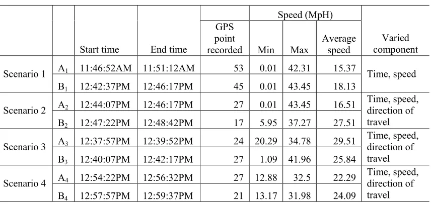
Scenario 1: Covered a drive on the same road segment in the same direction but at different times. The first drive lasted for about 4.33 minutes with an average speed of 15.37mph and total of 53 GPS points were recorded (Figure 3a and 3b). The second drive on this route in the same direction lasted for about 3.58 minutes with an average speed of 18.13mph and a total 45 GPS points were recorded. From Figures 4a and 4b, the variation in the speed of

travelled caused by road traffic conditions are evident, although there are periods of almost synchronised peaks and dips between both plots.

Scenario 2: Here the extracted trajectory data was recorded on the same road segments but from opposite travel directions on a single carriageway and at different times. On a typical single carriageway there is no central reservation or physical barrier separating the two directions of traffic flow.

Depending on the precision of the GPS, recorded points could snap about both lanes or points could be very close to each other even when recorded while on travelling on opposite lane. The first drive totalled about 2.25 minutes with average speed of 16.51mph and 28 points recorded while travel in the opposite direction lasted for about 1.25 minutes with an average speed of 27.51mph and 16 points were recorded.

Clearly, both speed-time plots (Figure 4a and b) for this scenario imply different road conditions and like in the earlier case does not conclude that both plots have any relation or where recorded from the same road.

Scenario 3: The extracted trajectory data for this scenario was recorded on the same road segments but from opposite travel directions and on a dual carriageway during different Figure 3: Speed-time plot for scenario 1: (a) first drive (b) second drive

time interval. The first drive lasted for about 1.91 minutes with an average travel speed of 29.51mph and total of 24 points were recorded while the return drive lasted for about 2.17 minutes with an average speed of 25.84mph and a total of 27 points were recorded. Overall the high speed regimes associated with dual carriageways are evident in both time-speed plots (Figures 5a and 5b).

Scenario 4: The extracted trajectory data for

this scenario was recorded on the same road segments but from opposite travel directions and on a dual carriageway during different time interval (Figure 6a and 6b). The first drive lasted for about 2 minutes with an average travel speed of 22.29mph and total of 27 points were recorded while the return drive lasted for about 2.10 minutes with an average speed of 24.09mph and a total of 21 points were recorded.

Table 2 shows the summary of the four scenarios and the varied component for each scenario. For instance, scenario 1, the varied component was time and travel speed and scenario 4 the time, speed and travel direction of travel (Table 2).

Clearly, relying on speed-time plot information alone would not be sufficient to determine on which road segments there are similar trajectories. For this purpose the

Snap-Drift Neural Network (SDNN) (Lee and Palmer-Brown, 2004) is used to group these features.

4. Snap-Drift Neural Network

(SDNN)

One of the strengths of the SDNN is the ability to adapt rapidly in a non-stationary environment where new patterns (new

Figure 5: Speed-time plot for scenario 3: (a) first drive (b) second drive

introduced over time. The learning process utilises a novel algorithm that performs a combination of fast, convergent, minimalist learning (snap) and more cautious learning

the data and more general holistic features. Snap and drift learning phases are combined within a learning system that toggles its learning style between the two modes.

On presentation of input data patterns at the input layer F1, the distributed SDNN (dSDNN) will learn to group them according to their features using snap-drift (Lee and Palmer-Brown, 2005). The neurons whose weight prototypes result in them receiving the highest activations are adapted. Weights are normalised weights so that in effect only the angle of the weight vector is adapted, meaning that a recognised feature is based on a particular ratio of values, rather than absolute values. The output winning neurons from dSDNN act as input data to the selection SDNN (sSDNN) module for the purpose of feature grouping and this layer is also subject to snap-drift learning.

The learning process is unlike error minimisation and maximum likelihood methods in MLPs and other kinds of

networks which perform optimization for classification or equivalents by for example pushing features in the direction that minimizes error, without any requirement for the feature to be statistically significant within the input data. In contrast, SDNN toggles its learning mode to find a rich set of features in the data and uses them to group the data into categories. Thus SDNN was used to group GPS-based trajectory data into the road types based on point-to-point properties like speed, horizontal and vertical curvature, acceleration, bearing and change in drive direction. Each weight vector is bounded by snap and drift: snapping gives the angle of the minimum values (on all dimensions) and drifting gives the average angle of the patterns grouped under the neuron. Snapping essentially provides an anchor vector pointing at the ‘bottom left

Table 2: Description of the spatio-temporal scenarios with varied components

Speed (MpH)

Start time End time

GPS point

recorded Min Max Average speed

Varied component

A1 11:46:52AM 11:51:12AM 53 0.01 42.31 15.37

Scenario 1

B1 12:42:37PM 12:46:17PM 45 0.01 43.45 18.13

Time, speed

A2 12:44:07PM 12:46:17PM 27 0.01 43.45 16.51

Scenario 2

B2 12:47:22PM 12:48:42PM 17 5.95 37.27 27.51

Time, speed, direction of travel

A3 12:37:57PM 12:39:52PM 24 20.29 34.78 29.51

Scenario 3

B3 12:40:07PM 12:42:17PM 27 1.09 41.96 25.84

Time, speed, direction of travel

A4 12:54:22PM 12:56:32PM 27 12.88 32.5 22.29

Scenario 4

B4 12:57:57PM 12:59:37PM 21 13.17 31.98 24.09

hand corner’ of the pattern group for which the neuron wins. This represents a feature common to all the patterns in the group and gives a high probability of rapid (in terms of epochs) convergence (both snap and drift are convergent, but snap is faster). Drifting, which uses Learning Vector Quantization (LVQ), tilts the vector towards the centroid angle of the group and ensures that an average, generalised feature is included in the final vector. The angular range of the pattern-group membership depends on the proximity of neighbouring groups (natural competition), but can also be controlled by adjusting a threshold on the weighted sum of inputs to the neurons. The output winning neurons from dSDNN act as input data to the selection SDNN (sSDNN) module for the purpose of feature grouping and this layer is also subject to snap-drift learning.

4.1. Inputs representation for SDNN

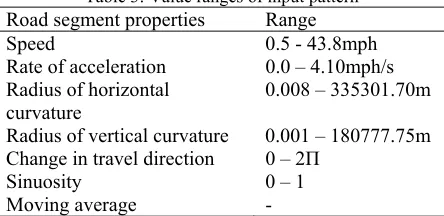
The input dataset for the SDNN and LVQ is composed of 7 variables represented by separate fields in the input vector. These are the speed between successive points, rate of acceleration between successive points, radius of horizontal and vertical curvature between three successive points and change in direction between successive points, sinuosity between three successive points and moving averages of these variables. Table 3 shows the values ranges of the 7 variables used.

Table 3: Value ranges of input pattern

Road segment properties Range

Speed 0.5 - 43.8mph

Rate of acceleration 0.0 – 4.10mph/s

Radius of horizontal

curvature 0.008 – 335301.70m

Radius of vertical curvature 0.001 – 180777.75m Change in travel direction 0 – 2Π

Sinuosity 0 – 1

Moving average -

5. Results

Figure 7a-d shows the features (winning nodes) that are present in each pair of scenario considered. For instance, in scenario 1, the SDNN groupings (winning node) shows that similar road features exist in both pairs of trajectory that make up scenario 1 although in varying composition (Figure 7a). Road features represented by winning nodes 1, 5, 6, 11, 14, 15 are present in both scenario trajectories signifying that although both trajectories were collected at different times under varying travel speed, key road features that are unique to the road segment travelled are encapsulated in the recorded trajectory. They simply occur in somewhat different proportions.

For scenario 2 – each pair of the trajectory data was recorded from opposite direction of the road segment at different times. The SDNN grouping reveals that both set of trajectory contain similar road features but in varying composition, these features are represented as winning nodes 1, 6, 11, 14 and 15. In this scenario, road feature represented by winning node 5 was only present in scenario 2b (Figure 7b). There is a positive correlation (0.71) between the winning nodes composition of each trajectory for scenario 2.

that could not reveal any similarity between the trajectory data for the considered

scenarios, the SDNN is able to reveal some

group them into unique winning nodes.

6. Conclusion

We have shown that while spatio-temporal variations associated with road traffic conditions affects the travel speed considerably, there are still road related features that are encapsulated in the recorded trajectory information that are unique to the road travelled. Clearly these features were not immediately visible in the speed information but the SDNN is able to capture the precise features that are unique to the travelled road. For our propose which is road updating, this result confirms that the SDNN is able to group road features such

that they correspond to the road class travelled even under changing road traffic conditions. The data used for the different scenarios was collected during one journey (11:43AM to 1: 05PM), it is possible that there was little variation in road traffic conditions around this time. The next step will be to record drive trajectory at different times and days to properly determine the working extremes of our approach.

Reference

EKPENYONG, F., BRIMICOMBE, A. & PALMER-BROWN, D. (2007a) Updating

Winning nodes

Frequency

Grouping Using Snap-Drift Neural Network.

Geographical Information Science Research Conference (GISRUK’07), 11-13th April 2007, Maynooth, Ireland.

EKPENYONG, F., PALMER-BROWN, D. & BRIMICOMBE, A. (2007b) Updating of Road Network Databases: Spatio-temporal Trajectory Grouping Using Snap-Drift Neural Network. 10th International

Conference on Engineering Applications of Neural Networks, 29-31 August 2007, Thessaloniki, Hellas.

GERKE, M., BUTENUTH, M., HEIPKE, C. & WILLRICH, F. (2004) Graph-supported verification of road databases. ISPRS Journal of Photogrammetry and Remote Sensing, 58, 152.

HOLZAPFEL, W., SOFSKY, M. & NEUSCHAEFER-RUBE, U. (2003) Road profile recognition for autonomous car navigation and Navstar GPS support.

Aerospace and Electronic Systems, IEEE Transactions on, 39, 2.

KLANG, D. (1998) Automatic detection of changes in road databases using satellite imagery. International Archives of Photogrammetry and Remote Sensing, 32 (Part 4), 293-298.

LEE, S. W. & PALMER-BROWN, D. (2005) Phrase recognition using snap-drift learning algorithm. The Internation Joint Conference on Neural Neural Networks (IJCNN' 2005). Montreal, Canada, 31st July - 4th August.

LEE, S. W., PALMER-BROWN, D. & ROADKNIGHT, C. M. (2004)

Performance-guided neural network for

management. Neurocomputing, 61, 5.

ZHANG, C. (2004a) Towards an operational system for automated updating of road databases by integration of imagery and geodata. ISPRS Journal of Photogrammetry and Remote Sensing, 58, 166.

ZHANG, Q. (2004b) A Framework for Road Change Detection and Map Updating.

International Archives of the