Electrophysiological Correlates of Processing Unattended Objects in Visual Cognition

ELECTROPHYSIOLOGICAL CORRELATES OF

PROCESSING UNATTENDED OBJECTS IN VISUAL

COGNITION

ELLEY WAKUI

A thesis submitted in partial fulfilment of the requirements of

the University of East London for the degree of Doctor of

Philosophy

Research is divided as to what degree visually unattended objects are processed (Lachter et al., 2008; Carrasco, 2011). The hybrid model of object recognition (Hummel, 2001) predicts that familiar objects are automatically recognised without attention. However under perceptual load theory (Lavie, 1995), when objects are rendered unattended due to exhausted attentional resources, they are not processed.

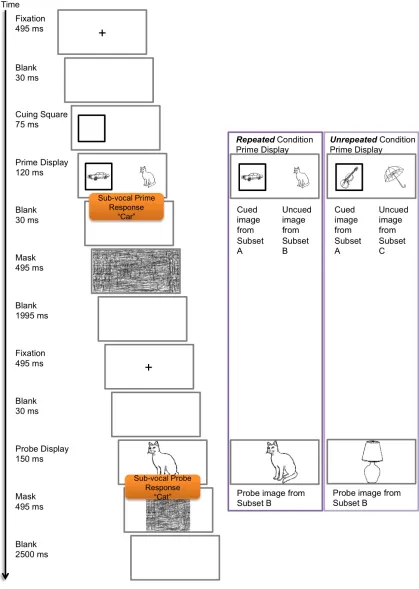
The present work examined the visual processing of images of everyday objects in a short-lag repetition-priming paradigm. In Experiments 1-3 attention was cued to the location of one of two objects in the first (prime) display, with the unattended sometimes repeated in the second (probe) display. ERP repetition effects were observed which were insensitive to changes in scale (Experiment 1) but sensitive to slight scrambling of the image (Experiment 2). Increasing perceptual load did not modulate these view-specific repetition effects (Experiment 3), consistent with the predictions of automatic holistic processing. In Experiments 4-7 a letter search task was used to render the flanking object image unattended under high load. In Experiment 5 distractor processing was observed in ERP even under high load. In Experiments 4, 6 and 7 a pattern of view

sensitive/insensitive and load sensitive/insensitive repetition effects on RT (Experiment 4) and ERP amplitude (Experiments 6, 7) were observed that were difficult to interpret under either the hybrid model or perceptual load theory, but may reflect fast view-based and slow view-independent processing of objects.

Chapter
1.
Introduction
and
Background ...15


1.1.
Basic
Rationale:
Why
Study
Unattended
Objects? ... 15


1.2.
Outline
and
Scope
of
the
Thesis ... 17


1.3.
What
is
Object
Recognition?... 19


1.4.
The
Neurobiology
of
the
Visual
System... 19


1.4.1
Two
Visual‐Streams
of
Object
Processing... 22


1.5.
The
Stages
of
Object
Processing... 25


1.5.1
Explicit
vs.
Implicit
Recognition ... 29


1.6.
Repetition­priming... 31


1.7.
View­sensitivity
of
Object
Recognition:
The
Viewpoint
Debate... 32


1.8.
The
Mental
Representation
of
Object
Shape... 33


1.8.1
Analytic
Representation/Theories
of
View‐independent
Recognition... 41


1.8.2
Holistic
Representation/Theories
of
View‐dependent
Recognition ... 45


1.9.
Accommodating
Both
Types
of
Representation
in
one
Model
of
Object
 Recognition ... 46


1.10.
The
Role
of
Attention
in
the
Binding
of
Object
Representations ... 51


1.11.
The
Hybrid
Model
of
Object
Recognition:
Incorporating
Both
Types
of
Binding
 and
Representation
in
one
Model
of
Object
Recognition ... 53


1.11.1
Description
of
JIM3... 57


1.11.2
Support
for
the
Hybrid
Model... 60


1.12.
The
Role
of
Attention
in
the
Two­systems
Account ... 63


1.13.
Attentional
Selection:
The
Question
of
Distinguishing
Attended
From
 Unattended... 65


1.14.
Perceptual
Load
Theory... 66


1.14.1
Support
for
Perceptual
Load
Theory ... 68


1.15.
Types
of
Attention:
Endogenous
vs.
Exogenous ... 70


1.16.
Reconciling
Perceptual
Load
Theory
and
the
Hybrid
Model
of
Object
 Recognition ... 71


1.17.
Models
of
Top­down
Guided
Attention
Object
Recognition... 73


2.1.
EEG
in
Cognitive
Neuroscience... 82


2.1.1
Electrogenesis
of
EEG... 83


2.1.2
Derivation
of
ERP... 85


2.1.3
Interpretation
of
ERP ... 86


2.1.4
Visual
ERP
components... 89


2.2.
Review
of
ERP
in
Object
Recognition
and
Spatial
Attention... 92


2.2.1
ERP
and
Object
Processing ... 94


2.2.2
ERP
Repetition
Effects ...101


2.3.
Acquisition
of
EEG
and
General
Methods
for
Thesis ...114


2.3.1
Ethics...114


2.3.2
Recording
Procedures...114


2.3.3
ERP
Data
Pre‐Processing...117


2.3.4
Statistical
Analysis...120


Chapter
3.
Experiment
1:
ERP
Repetition
Effects
from
Spatially
Unattended
 Objects... 123


3.1.
Introduction...123


3.2.
Participants...126


3.3.
Stimuli
&
Design ...126


3.4.
Procedure ...128


3.5.
Behavioural
Results ...131


3.6.
ERP
Results ...131


3.6.1
Probe‐locked
P1 ...134


3.6.2
Probe‐locked
N1...134


3.6.3
Probe‐locked
N250 ...136


3.7.
Experiment
1:
Summary
and
Discussion ...136


Chapter
4.
Experiment
2:
View­sensitivity
of
ERP
Repetition
Effects
from
 Spatially
Unattended
Objects
to
Split
images ... 138


4.1.
Introduction...138


4.2.
Participants...141


4.6.
ERP
Results ...146


4.6.1
Probe‐locked
ERP ...146


4.6.2
Comparison
of
Scalp
Topography
of
Repetition
effects
for
Experiments
1
and
2 ...150


4.6.3
Prime‐locked
ERP ...151


4.7.
Experiment
2:
Summary
and
Discussion ...154


Chapter
5.
Experiment
3:
The
Effect
of
Perceptual
Load
on
the
ERP
Repetition
 Effects
from
Spatially
Uncued
Objects... 159


5.1.
Introduction...159


5.2.
Participants...162


5.3.
Stimuli
&
Design ...163


5.4.
Procedure ...166


5.5.
Behavioural
Results ...166


5.6.
ERP
Results ...167


5.6.1
Probe‐locked
ERP ...167


5.6.2
Prime‐locked
ERP ...172


5.7.
Experiment
3:
Summary
and
Discussion ...175


5.8.
Summary
of
Experiments
1­3 ...177


Chapter
6.
Experiment
4:
The
Effect
of
Perceptual
Load
and
View
(split
 images)
from
Task­irrelevant
Peripheral
Images
on
Behavioural
Priming
 Using
a
Letter
Search
Task ... 180


6.1.
Introduction...180


6.2.
Participants...183


6.3.
Stimuli
&
Design ...183


6.4.
Procedure ...185


6.5.
Behavioural
Results ...188


6.6.
Eye
tracking
Results...190


6.7.
Experiment
4:
Summary
and
Discussion ...192


7.3.
Stimuli
&
Design ...197


7.4.
Procedure ...199


7.5.
Behavioural
Results ...201


7.6.
ERP
Results ...202


7.6.1
N1
Amplitude...207


7.6.2
N2pc...208


7.7.
Experiment
5:
Summary
&
Discussion...211


Chapter
8.
Experiment
6:
The
Effects
of
Perceptual
Load
and
View
(split
 images)
on
ERP
Repetition
Effects
from
Task­irrelevant
Peripheral
Images
 Using
a
Letter
Search
Task. ... 215


8.1.
Introduction...215


8.2.
Participants...216


8.3.
Stimuli
&
Design ...217


8.4.
Procedure ...219


8.5.
Behavioural
Results ...221


8.6.
ERP
Results ...223


8.6.1
Probe‐locked
P1 ...225


8.6.2
N1...228


8.6.3
N250:
230‐270
time
window...230


8.6.4
N250:
270‐310
time
window...232


8.6.5
Prime‐locked
ERP ...232


8.7.
Experiment
6:
Summary
and
Discussion ...234


Chapter
9.
Experiment
7:
The
Effects
of
Perceptual
Load
and
View
(inverted
 images)
on
ERP
Repetition
Effects
from
Task­irrelevant
Peripheral
Images
 Using
a
Letter
Search
Task ... 238


9.1.
Introduction...238


9.2.
Participants...239


9.3.
Stimuli
&
Design ...239


9.4.
Procedure ...242


9.6.2
Probe‐locked
N1...249


9.6.3
Probe‐locked
N250:
200‐240
ms ...251


9.6.4
Probe‐locked
N250:
240‐270ms ...253


9.6.5
Prime‐Locked
ERP...255


9.7.
Experiment
7:
Summary
and
Discussion ...258


Chapter
10.
General
Discussion... 261


10.1.
Research
Motivation...261


10.1.1
Main
Findings...262


10.2.
Overview
of
Experiments
and
Main
Results...263


10.3.
Implications
for
Object
Recognition ...269


10.3.1
ERP
Repetition
Effects
from
Unattended
Objects ...269


10.3.2
View‐sensitivity
of
ERP
Repetition
Effects
from
Unattended
Objects ...275


10.3.3
Summary
of
Implications
for
Object
Recognition ...279


10.4.
Implications
for
Visual
Attention...280


10.4.1
Automatic
and
Pre‐attentive
Processing ...280


10.4.2
Early
vs.
Late
Selection ...281


10.4.3
Selection
Mechanisms
in
Attention ...284


10.5.
Integrating
ERP
Repetition
Effects
with
the
Hybrid
Model
of
Object
 Recognition
and
Perceptual
Load
Theory ...287


10.5.1
The
Role
of
Attention
in
Visual
Short‐Term
Memory
(VSTM)...291


10.6.
Limitations
and
Further
Work...293


10.7.
Conclusions...294


Appendix
I:
Ethics
and
Examples
of
Participant
Introduction
Letter,
Consent
 and
Debrief
Forms ... 318


Confirmation
of
UEL
Ethics
Approval...318


Example
Introduction
Letter,
Consent
Form,
Debrief ...319


Appendix
IV:
Prime­locked
ERP
Analyses
for
P1
and
N1
for
Experiments
6
&
7

... 340


Appendix
V:
Stimulus
Lists
for
Experiment
1 ... 345


Appendix
VI:
Stimulus
Lists
for
Experiment
2... 347


Appendix
VII:
Stimulus
Lists
for
Experiment
3 ... 350


Appendix
VIII:
Stimulus
Lists
for
Experiment
4... 353


Appendix
IX:
Stimulus
Lists
for
Experiment
5... 355


Appendix
X:
Stimulus
Lists
for
Experiment
6 ... 356


Appendix
XI:
Stimulus
Lists
for
Experiment
7... 359


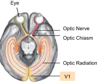
Figure
1‐1:
Illustration
of
human
early
visual
areas
(adapted
from
Logothetis,
1999)... 21


Figure
1‐2:
Hierarchical
visual
areas
in
cortex
(adapted
from
Logothetis,
1999)... 22


Figure
1‐3:
Schematic
of
the
dorsal
and
ventral
visual
pathways
in
human
cortex
adapted
from
 Goodale
&
Westwood
(2004).
Also
shown
is
the
subcortical,
retinotectal,
pathway... 24


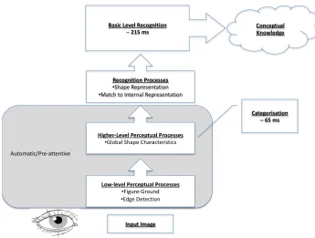
Figure
1‐4:
Schematic
of
the
levels
of
object
processing. ... 29


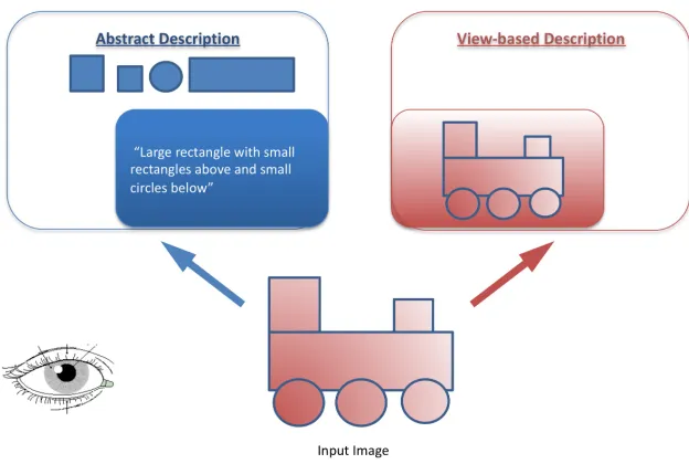
Figure
1‐5:
Simplified
examples
of
a
view‐based
description
and
an
abstract
description
of
an
image. ... 34


Figure
1‐6:
Examples
of
volumetric
elements
and
examples
of
assembly
into
a
cup
and
bucket. ... 35


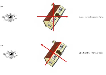
Figure
1‐7:
Illustration
of
(a)
viewer‐centred
and
(b)
object‐centred
reference
frames.
Object
image
 from
the
stimulus
set
of
Rossion
and
Pourtois
(2004). ... 36


Figure
1‐8:
An
example
of
spatial
relations
between
the
house‐parts
of
window
and
door
defined
by
 (a)
coordinates
and
(b)
categorical
relations.
Object
image
from
the
stimulus
set
of
Rossion
and
 Pourtois
(2004)... 37


Figure
1‐9:
Schematic
of
analytic
and
holistic
descriptions. ... 39


Figure
1‐10:
Recognition
of
an
object
upon
a
view‐change... 40


Figure
1‐11:
Generalised
cylinders
(adapted
from
Marr
&
Nishihara,
1978). ... 42


Figure
1‐12:
Examples
of
geons
(adapted
from
Biederman,
1987)... 43


Figure
1‐13:
Different
objects
based
on
similar
geons
but
different
spatial
configurations
(adapted
 from
Biederman,
1987). ... 43


Figure
1‐14:
Schematic
of
JIM3
(adapted
from
Hummel,
2001).
The
red
boxes
correspond
to
the
 holistic,
unattended,
route
and
the
blue
boxes
to
the
analytic,
attended,
route
of
recognition... 58


Figure
1‐15:
Example
of
a
prime
and
probe
display
for
a
spatial
cuing
priming
task. ... 61


Figure
1‐16:
Typical
presentation
for
a
low
(a)
and
high
(b)
perceptual
load
task
from
Lavie
(2005). ... 69


Figure
2‐1:
Illustration
of
processes
of
electrogenesis
of
EEG... 84


Figure
2‐2:
Extracting
an
ERP
from
raw
EEG
in
two
experimental
conditions
(adapted
from
Luck,
 2005)... 85


Figure
2‐3:
Example
of
an
ERP
waveform
adapted
from
McFadden
and
Rojas
(2013)... 86


Figure
2‐4:
Summation
of
different
ERP
latent
components
result
in
the
same
profile
for
the
observed
 waveform
(adapted
from
Luck,
2005). ... 88


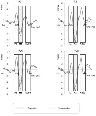
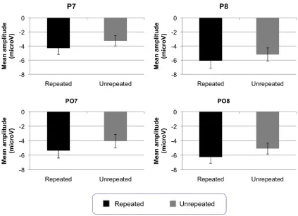
Figure
3‐3:
Grand‐averaged
probe‐locked
ERP
waveforms
for
30
Hz
low‐pass
filtered
data
for
each
 experimental
condition
for
P7,
P8,
PO7
and
PO8
for
Experiment
1.
P1,
N1
and
N250
time
 windows
are
marked,
where
these
boxes
are
grey
indicates
that
statistically
significant
 repetition
effects
were
observed
in
these
time
windows.
For
those
time
windows
where
 statistically
significant
effects
were
found,
bar
charts
showing
mean
amplitudes
are
presented
 separately
below... 133
 Figure
3‐4:
Probe‐locked
N1
mean
amplitudes
±1
standard
error
bars
for
each
electrode
analysed
for


Experiment
1 ... 135
 Figure
3‐5:
Probe‐locked
difference
topomaps
between
130–200
ms
post‐stimulus
onset
in
10
ms


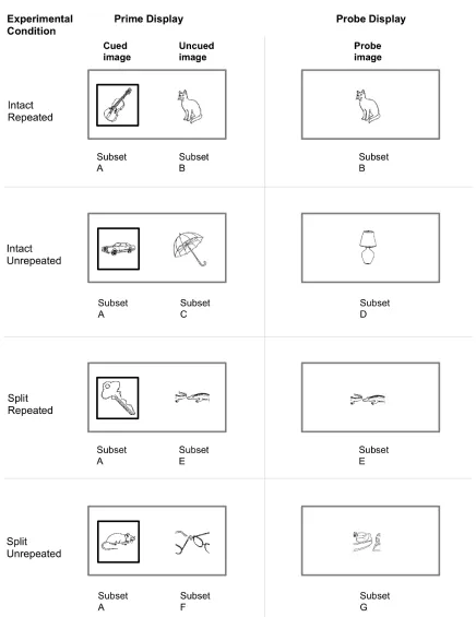
steps
for
Experiment
1... 135
 Figure
4‐1:
Example
of
a
split
image
stimulus... 139
 Figure
4‐2:
Schematic
of
conditions
and
stimulus
subsets
for
the
first
participant
(counterbalancing


of
sets
B
–
G)
in
Experiment
2... 142
 Figure
4‐3:
Mean
probe
RT
for
each
condition
±1
standard
error
bars
for
Experiment
2 ... 145
 Figure
4‐4:
Grand‐averaged
probe‐locked
ERP
waveforms
for
30
Hz
low‐pass
filtered
data
for
each


experimental
condition
for
P7,
P8,
PO7
and
PO8
for
Experiment
2.
P1,
N1
and
N250
time
 windows
are
marked,
where
these
boxes
are
grey
indicates
that
statistically
significant
 repetition
effects
were
observed
in
these
time
windows.
For
those
time
windows
where
 statistically
significant
effects
were
found,
bar
charts
showing
mean
amplitudes
are
presented
 separately
below... 147
 Figure
4‐5:
Probe‐locked
N250
mean
amplitudes
±1
standard
error
bars
at
each
electrode
for


Experiment
2 ... 149
 Figure
4‐6:
Probe‐locked
difference
topomaps
between
220‐380
ms
post‐stimulus
onset
in
20
ms


steps
for
Experiment
2... 150
 Figure
4‐7:
Comparison
of
difference
topomaps
from
(a)
Experiment
1
and
(b)
Experiment
2.
Note


different
scales
to
maximise
appearance
of
the
effect
of
repetition
for
comparison
of
location
 rather
than
magnitude. ... 151
 Figure
4‐8:
Grand‐averaged
prime‐locked
contralateral
and
ipsilateral
waveforms
for
30
Hz
low‐pass


filtered
data
for
each
experimental
condition
for
P7,
P8,
PO7
and
PO8
for
Experiment
2.
The
 time
window
for
the
N2pc
is
marked,
where
this
is
grey
indicates
that
a
statistically
significant
 N2pc
was
observed... 153
 Figure
5‐1:
Schematic
of
conditions
and
stimulus
subsets
(counterbalanced)
for
the
first
participant


time
windows
are
marked,
where
these
boxes
are
grey
indicates
that
statistically
significant
 repetition
effects
were
observed
in
these
time
windows.
For
those
time
windows
where
 statistically
significant
effects
were
found,
bar
charts
showing
mean
amplitudes
are
presented


separately
below... 169


Figure
5‐4:
Probe‐locked
N1
mean
amplitudes,
±1
standard
error
bars
for
Experiment
3. ... 171


Figure
5‐5:
Grand‐averaged
prime‐locked
contralateral
and
ipsilateral
waveforms
for
30
Hz
low‐pass
 filtered
data
for
each
experimental
condition
for
P7,
P8,
PO7,
PO8,
O1
and
O2
for
Experiment
3.
 The
time
window
for
the
N2pc
is
marked,
where
this
is
grey
indicates
that
a
statistically
 significant
N2pc
was
observed... 174


Figure
6‐1:
Schematic
of
conditions
and
stimulus
subsets
for
the
first
participant
in
Experiment
4 184
 Figure
6‐2:
Example
trial
display
sequence
for
Experiment
4. ... 187


Figure
6‐3:
Mean
probe
RT
for
each
condition
±1
standard
error
bars
for
Experiment
4. ... 190


Figure
6‐4:
Location
and
duration
of
fixations
from
all
participants
overlaid
on
prime
presentation
 display
for
Experiment
4.
The
colour
represents
the
duration
(sec)
of
each
fixation
and
the
 location
is
given
in
eye‐tracker
horizontal
(x‐axis)
and
vertical
(y‐axis)
units ... 191


Figure
6‐5:
Percentage
number
of
all
fixations
(over
50
ms)
for
all
participants
in
each
defined
area
of
 interest
of
the
prime
presentation
display
for
Experiment
4.
NB
for
the
areas
of
interest
of
left
 and
right
images
there
were
no
fixations. ... 191


Figure
7‐1:
Schematic
of
conditions
and
stimulus
subsets
for
Experiment
5... 199


Figure
7‐2:
Example
trial
display
sequence
for
Experiment
5. ... 200


Figure
7‐3:
Mean
RT
for
each
condition
±1
standard
error
bars
for
Experiment
5... 202


Figure
7‐4:
Grand
averaged
ERP
contralateral
and
ipsilateral
waveforms
locked
to
stimulus
onset
for
 each
condition
of
load
for
30
Hz
low‐pass
filtered
data
for
(a)
target
and
distractor
near
(b)
 target
and
distractor
far
(c)
no
distractor
present
for
P7,
P8,
PO7,
PO8,
O1
and
O2
for
 Experiment
5.
The
time
window
for
the
N2pc
is
indicated... 206


Figure
7‐5:
Difference
topomaps
for
left‐right
visual
field
between
220‐280
ms
post‐stimulus
onset
in
 20
ms
steps
for
each
condition
for
Experiment
5. ... 211


Figure
8‐1:
Schematic
of
conditions
and
stimulus
subsets
for
the
first
participant
in ... 218


Figure
8‐2:
Example
trial
display
sequence
for
Experiment
6. ... 220


Figure
8‐3:
Mean
probe
RT
for
each
condition
±1
standard
error
bars
for
Experiment
6 ... 222
 Figure
8‐4:
Grand‐averaged
probe‐locked
ERP
waveforms
for
30
Hz
low‐pass
filtered
data
for
each


Figure
8‐5:
Probe‐locked
P1
mean
amplitudes
±1
standard
error
bars
for
Experiment
6... 227
 Figure
8‐6:
Probe‐locked
N1
mean
amplitudes
±1
standard
error
bars
for
Experiment
6. ... 229
 Figure
8‐7:
Probe‐locked
N250
(230‐270
ms)
mean
amplitudes
±1
standard
error
bars
for


Experiment
6 ... 231
 Figure
8‐8:
Grand‐averaged
prime‐locked
contralateral
and
ipsilateral
waveforms
for
30
Hz
low‐pass


filtered
data
for
each
experimental
condition
for
P7,
P8,
PO7,
PO8,
O1
and
O2
for
Experiment
6.
 The
time
window
for
the
N2pc
is
marked,
where
this
is
grey
indicates
that
a
statistically


significant
N2pc
was
observed... 233
 Figure
9‐1:Schematic
of
conditions
and
stimulus
subsets
for
the
first
participant
in
Experiment
7. 241
 Figure
9‐2:
Mean
probe
RT
for
each
condition
±1
standard
error
bars
for
Experiment
7. ... 244
 Figure
9‐3:
Grand‐averaged
probe‐locked
ERP
waveforms
for
30
Hz
low‐pass
filtered
data
for
each


experimental
condition
for
P7,
P8,
PO7,
PO8,
O1
and
O2
for
Experiment
7.
P1,
N1
and
N250(a
&
 b)
time
windows
are
marked,
where
these
boxes
are
grey
indicates
that
statistically
significant
 repetition
effects
were
observed
in
these
time
windows.
For
those
time
windows
where
 statistically
significant
effects
were
found,
bar
charts
showing
mean
amplitudes
are
presented
 separately
below... 246
 Figure
9‐4:
Probe‐locked
P1
mean
amplitudes
±1
standard
error
bars
for
Experiment
7... 248
 Figure
9‐5:
Probe‐locked
N1
mean
amplitudes
±1
standard
error
bars
for
Experiment
7. ... 250
 Figure
9‐6:
Probe‐locked
N250
(200‐240
ms)
mean
amplitudes
±1
standard
error
bars
for


Experiment
7... 252
 Figure
9‐7:
Probe‐locked
N250
(240‐270
ms)
mean
amplitudes
±1
standard
error
bars
for


Experiment
7... 254
 Figure
9‐8:
Grand‐averaged
prime‐locked
contralateral
and
ipsilateral
waveforms
for
30
Hz
low‐pass


filtered
data
for
each
experimental
condition
for
P7,
P8,
PO7,
PO8,
O1
and
O2
for
Experiment
7.
 The
time
window
for
the
N2pc
is
marked,
where
this
is
grey
indicates
that
a
statistically


Table
3‐1:
Counterbalancing
of
object
subsets
for
the
first
three
participants
in
Experiment
1... 128
 Table
4‐1:
Counterbalancing
of
object
subsets
for
the
first
three
participants
in
Experiment
2... 143
 Table
5‐1:
Counterbalancing
of
object
subsets
for
the
first
three
participants
in
Experiment
3... 165
 Table
10‐1:
Summary
of
experiments
with
outcomes.
Note:
all
effects
concern
unattended
(flanker)


objects,
with
the
manipulation
of
view
and
attention
(Load)
in
the
prime
display,
except


Acknowledgements

There are many people that I would like to thank for their help, guidance and good cheer along the way.

My supervisory ‘super-team’ of Volker Thoma (DoS), Melanie Vitkovitch and Ashok Jansari for always listening with patience and offering helpful feedback. Thank you for helping me to try and understand what it is that I want to say! And thanks to reviewers Lynne Dawkins and Mary Spiller for my annual dose of really good advice, and James Walsh too. Thanks to John Hummel for his answering questions on the hybrid model. I asked everyone who even mentioned EEG for help at some point, and I am very grateful for the wise words of Angie Gosling, Silvia Rigato and Prezemek Tomalski. Also Jose van Velzen and Luke and Job at Goldsmiths when I camped out there during the

Olympics. And Gaynor and Dritan at EGI especially for responding to my early panicky emails.

At UEL, many thanks to Kevin, Pete, Andy and Ambi for always finding a way to fix the lab and with such good humour and calm. Also Anita Potton for her instruction in using the eye-tracking lab. And Shaila and Will for always knowing how things work.

Thanks also to all who participated in my studies.

Thanks to those friends who have passed through the research suite and have always made Stratford a shinier happier place –Dee, Caroline, Elisa, Elliott, Shani, Haiko, Jerry, Friederike and my fellow students Nesrin, Anna, Francesca and Paula.

Chapter 1.

Introduction and Background

1.1.Basic Rationale: Why Study Unattended Objects?

Consider driving in a new city without a navigation system. It is important to both navigate the traffic safely, but at the same time follow the signs to avoid getting lost. To stay on the right route, do we need to actively direct our attention away from the traffic to the signs themselves, or is any recognition of the information displayed still possible without attention? Does it make a difference if the information is displayed on the signs in a familiar way? Does the amount of traffic or displays on the dashboard (i.e. ‘clutter’ in a scene) affect how much information we can gain from the street signs?

The example above illustrates the interaction between attention and object recognition: we must attend to the task of navigating through traffic and we must also recognise the information on the street signs in order not to get lost. These tasks may interact; for example, attending more or less to the traffic may determine how well we can process objects in the periphery. The topic of this thesis concerns the way in which these aspects of attention and object recognition interact in our visual cognition. Indeed, Walther and Koch (2007) have argued that understanding the interaction between attention and object recognition is a requirement for constructing a full model of human visual subjective experience.

One model of the few models of object recognition that makes clear predictions on the role of attention in object recognition is the hybrid model of Hummel (2001). It proposes that the shape information of attended and unattended objects are represented in a

qualitatively different way, and that recognition is possible without attention for objects in familiar views.

The successful recognition of objects can be measured by repetition-priming. In such a paradigm, the first presentation of the object is termed the ‘prime’ display and the second is termed the ‘probe’. Priming is measured behaviourally as the difference in the naming accuracy or decrease in the naming time of an object at the probe display due to it having been presented previously at the prime display, compared to a baseline object that has not been seen previously at all (Bartram, 1976; Schacter, Delaney & Merikle, 1990). Priming has been described as “likely to be one of the most basic expressions of memory,

influencing how we perceive and interpret the world” (Henson, 2009, p.1055) and priming is therefore an appropriate paradigm to examine the link between attention and format of object representations in memory. Thus all except one of the experiments in this thesis were based on a short-lag repetition-priming paradigm.

This thesis directly examines the effects of view on the visual processing of unattended objects, extending the current literature by using electroencephalographic (EEG) techniques. EEG are scalp-recorded voltage-potential changes that are associated with neural activity. By comparing the EEG locked to a certain event (for example a stimulus onset) an event-related potential (ERP) can be extracted. The ERPs for different

This thesis concerns human visual object recognition, and particularly whether visual processing of objects can occur without attention. Here, an object is defined as an everyday object easily recognisable from its image displayed in a canonical view. All images used in the research studies for this thesis were black and white line drawings. ERP repetition-priming studies form the basis of the experimental work described here.

1.2.Outline and Scope of the Thesis

Chapter 1 of this thesis provides a background to the relevant areas of object recognition and selective attention to contextualise the rationale for the overall research questions. It begins with a discussion of the basic problems in understanding object recognition and how certain types of models have attempted to resolve these by proposing different ways in which we represent objects in long-term memory (LTM). It will be argued that the instances of these representations are restricted by whether objects are placed under attention or not. Rather than a full discussion of all object recognition models, one model that directly integrates the role of attention into object recognition is highlighted here: the hybrid model of object recognition (Hummel, 2001). This model provides the framework required for testing the specific properties of the recognition of unattended objects as is the aim of this thesis. The scope of this thesis is limited to the recognition of single non-face objects, rather than that involving multiple objects as in scene recognition.

demand for a central task is low, ‘ignored’ objects still receive residual attention, and are processed. Thus, these two theories are used as the framework to address our research questions: The hybrid model of object recognition will guide the tests of whether an unattended object can be recognised, and whether unattended objects can be recognised across changes in view. The perceptual load theory of attention is employed to ask how robust this processing of unattended objects is to another method of modulating attention: perceptual load. The aim of Chapter 1 is to provide the background for the overall

research questions for the thesis, while the literature review specific to the relevant ERP studies used to form the experimental hypotheses is reserved for Chapter 2.

Chapter 2 also provides the specific experimental approach to the research questions and the choice of task. Studies testing both the hybrid model and perceptual load theory have used priming paradigms in an object-naming task. In this thesis repetition-priming is also chosen for all but one of the experimental tests, here modified for ERP and eye-tracking measurements. Some theoretical background on the acquisition of ERP will be given and this is followed by an overview of the literature on observations of relevant ERP effects that provide the explicit basis for the specific experimental

predictions of this thesis. The general methods for the acquisition and analysis of the data for this thesis are described in the second part of Chapter 2. Eye-tracking measures are used in Experiment 4 and these are outlined in that chapter.

1.3.What is Object Recognition?

Recognising objects forms such an essential, and usually effortless, part of our daily experience that the complexity of understanding the processes involved can be easily overlooked (Humphreys, Riddoch & Price, 1997). Keysers, Xiao, Földiák and Perrett (2001) note that the mechanisms underlying biological object recognition are not well understood, and equally its implementation in computer models is still not

straightforward (DiCarlo & Cox, 2007; Pinto et al., 2008).

Put simply, functional accounts of object recognition must relate how, on first encountering an object, its retinal image is encoded (described) into an internal

representation. The accounts must then also explain the processes that, on a subsequent encounter with the same object, lead to a successful match of the input retinal image of an object to its description in long-term memory, resulting in recognition. Therefore, the properties of recognition rely upon how we internally represent objects (Marr, 1982), and, as stated by Riesenhuber (2000), any theoretical models of human object recognition must be constrained by neurobiology. Most models of object recognition do indeed follow the functional hierarchy of the visual areas of the brain, which is outlined below. A detailed account of the neurobiology of the visual system will not be given here, and the focus will rather be to describe the route of light from an input image through the brain until it reaches areas associated with object recognition. The emphasis of this chapter is a functional approach to the stages of object processing.

1.4.The Neurobiology of the Visual System

optic tract and lead to the lateral geniculate nuclei (LGN), which are small bilateral areas of the thalamus at which 80% of the axons terminate. These LGN consist of 6 layers, of which the top four layers extend mainly from the fovea and are termed parvocellular from the Latin “parvus” meaning small, with respect to the magnocellular (“magnus” meaning large) bottom two layers which extend mainly from the periphery. The magnocellular cells (M-cells) and parvocellular cells (P-cells),1 _{have been found to transmit different} types of visual information (e.g. Merigan, Katz & Maunsell, 1991; Bullier, 1995; Bar et al., 2006). The properties relating to M-cells and P-cells are maintained along the output axons (termed the optic radiation) leading to the primary visual area of cortex, V1 (Brodman area 17). V1 is the first point at which information from both eyes is

combined. It is known as striate (i.e. layered/striped) cortex, and is composed of 6 layers. The LGN axons terminate in the 4th layer (which is itself further sub-striated).

These early visual areas in primary cortex are considered to be retinotopic. That is, the cells contribute to a one-to-one map of the visual field, preserving topographic (location) information directly. This is illustrated by the instances of scotoma, in which damage to specific areas in V1 causes a location-specific blindspot on the retina (Wickens, 2009). These earliest visual areas are also known to be orientation-sensitive, with simple cells with small receptive fields tuned to different orientations (Hubel & Wiesel, 1962, 1977).

1

The M- and P- cells actually represent only 20% of the total input to LGN from the retina, with the majority actually from the brainstem and visual cortex, which may be involved with top-down feedback for example to sharpen the visual image, or to control jumpiness from saccadic

Figure 1-1: Illustration of human early visual areas (adapted from Logothetis, 1999).

The primary visual cortex then leads to the secondary, extrastriate, regions of visual cortex (V2, V3, V4 & V5, as shown in Figure 1-2). These regions are associated with the higher order processes of object recognition (although see Tong, 2003, for discussion of recognition linked directly with V1). Progressing through the hierarchical regions of the visual system, the receptive field sizes increase and also begin to respond to more complex stimuli (Kravitz, Vinson & Baker, 2008; Logothetis, Pauls, Bülthoff & Poggio, 1994).

Figure 1-2: Hierarchical visual areas in cortex (adapted from Logothetis, 1999).

It has been shown that there are two pathways for the flow of visual information through secondary cortex, one is a more dorsal route and the other more ventral (e.g. Goodale & Milner, 2006), and this is briefly described below.

1.4.1 Two Visual-Streams of Object Processing

The divergence of two distinct pathways for visual information from about V2 in the cortex is the basis of the influential two visual-systems approach (Goodale & Milner, 1992; Schneider, 1969; Ungerleider & Mishkin, 1982), which dissociates a ventral (from striate to inferotemporal cortex) stream from a dorsal stream (from striate to posterior parietal cortex) of visual processing. These streams are considered to be functionally separated either due to receiving different types of visual information (Ungerleider & Mishkin, 1982) or due to different processing of the same input information (Goodale & Milner, 1992).

Haxby (1994) described the evidence for these routes based on the results of studies on monkeys with lesions to temporal (dorsal) and parietal (ventral) cortical areas performing an object discrimination task and a landmark discrimination task. The monkeys were rewarded on choosing a familiarised object or location respective to the task condition. They were then lesioned, and tested on their retention of the task demands. Inferior temporal lesions were associated with reduced performance on visual discrimination based on pattern, object shape and colour, but no deficit on visuo-spatial tasks such as guided reaching (Gaffan, Harrison & Gaffan, 1986). In contrast, parietal lesions resulted in reduced visuo-spatial performance, but no deficits in visual discrimination (Mishkin & Ungerleider, 1982). Ungerleider and Haxby also linked these properties to human visual areas, describing how deficits of visuo-spatial performance or recognition were linked to occipito-parietal and occipito-temporal lesions respectively by postmortem (Newcombe, Ratcliff & Damasio, 1987). Ungerleider and Haxby also claimed that certain neurological conditions offer further support to the two routes hypothesis. One example was of object agnosia and prosopagnosia (where patients are able to detect an object or face without being able to recognise it) observed after occipito-temporal lesions. Another example was of the spatial cognition problems such as optic ataxia (where patients are able to identify an object but are unable to move their hand towards it effectively) that are observed after occipito-parietal lesions.

Goodale and Milner (2008) suggested that although both routes process location and structure information, the way that they process the information and then transmit it differs according to the goals of ‘vision for perception’ in the ‘what’ route or ‘vision for action’ in the ‘how’ route (Brown, Moore & Rosenbaum, 2002; Goodale & Milner, 1992; Milner & Goodale, 2008). The dorsal stream transforms ‘moment-to-moment’

(bilateral nuclei in the thalamus) separately feed the dorsal and ventral cortical routes. The subcortical pathway has been linked with the sensitivity to salient stimuli such as faces (Pasley, Mayes & Schultz, 2004), rather than in object recognition as is the case for the higher cortical areas. The three streams are illustrated in Figure 1-3.

Figure 1-3: Schematic of the dorsal and ventral visual pathways in human cortex adapted from Goodale & Westwood (2004). Also shown is the subcortical, retinotectal, pathway.

Reviews of the two-streams account can be found in Cardoso-Leite and Gorea (2010), Goodale and Milner (2006), Milner and Goodale (2008) and Westwood and Goodale (2011). Some authors have suggested that there is rather some integration of the two routes (Farivar, 2009; Grill-Spector, 2003), or a three-pathway model (Kravitz, Saleem, Baker & Mishkin, 2011), or even a patchwork model of about 40 inter-connected visual areas (de Haan & Cowey, 2011). The dissociation between the ventral and dorsal

demonstrated that cortical areas in the dorsal and ventral stream map onto one hybrid model of object recognition (Hummel, 2001), which will be discussed in Section 1.11.

1.5.The Stages of Object Processing

The stages of visual processing that are required for the recognition of an object can be broadly separated into perception and recognition (e.g. Schendan & Kutas, 2003; Lamberts & Freeman, 1999). Perceptual processes (occurring within around 200 ms of the presentation of the object) are concerned with the first detection and encoding of the visual scene by our sensory systems (the eye and striate cortex). Such processing includes basic figure-ground segregation, that is, the separation of the to-be-identified object from the background, and also some extraction of low-level visual features such as colour, edges and contour. In contrast, recognition processes are generally considered to be higher order processes, both functionally, for example, concerned more with the

matching of the percept resulting from the perceptual processes to an object description in long-term memory, and also neurologically, involving extra-striate cortex

(Riesenhuber & Poggio, 2000). The object descriptions may then lead to the activation of further conceptual associations with the object, for example linking an image of a cat to the knowledge that it is an animal, and that the word ‘cat’ begins with the letter ‘c’ in English, and so forth. The differences in perceptual and conceptual descriptions and the networks of associations are discussed further in Barsalou (2008) and Barsalou, Spivey and McRae (2012).

share some characteristics: chairs, desks, lamps have quite different features) or the more specific subordinate level (e.g. kitchen chairs compared to armchairs).

Analogous to this hierarchy of levels of naming, different levels of visual processing can be associated with the information required for a response appropriate to each of these levels. For example, categorisation can be demonstrated by those tasks such as simply asking participants whether they recognise an object or not, this being the basis of old/new (same/different) recognition paradigm. In such categorisation tasks participants may be taken through a learning phase and then asked whether certain stimuli have been presented to them previously. Other examples of categorisation tasks are judgements of stimuli as living vs. non-living, or size judgement (whether or not it fits in a shoe box e.g. Henson, Rylands, Ross, Vuilleumeir & Rugg, 2004) and gender categorisation. It has been suggested that such categorisation relies on the lower-level visual properties of an image. For example Lamberts, Brockdorff and Heit (2002) have associated perceptual processes with those required for an old/new response. Further, it has been suggested that categorisation may only require low-level perceptual processing of the ‘gist’ of an object for recognition e.g. by Thorpe, Fize and Marlot (1996). In their study they showed that categorisation is a very fast process, specifically that it is possible to identify whether there is an animal presented in a natural scene after only about 150 ms after a very brief presentation (20 ms). Thorpe et al. took this as an indication of fast feed-forward gist processing, arguing that there was insufficient time for top-down influence.2

The study by Thorpe et al. (1996) demonstrated the fast categorisation of whether an animal was present or not, but the level of the knowledge of that animal is not completely clear. On one hand, it may be that the animal was classified as ‘animal’. On the other hand, there may have been access to its basic level name ‘tiger’. Alternatively, the task may be regarded as detection of an animal from the background. Grill-Spector and Kanwisher (2005) have suggested that detection is as fast as categorisation, but in their study, the categorisation task required the participants to name objects at their basic level. Detection was tested by participants’ responses to everyday objects vs. textures. For the categorisation task participants had to name the objects at basic level across ten

2

categories, for example ‘face’, ‘dog’. For the identification task, participants had to name the same objects but at the subordinate level, for example ‘Harrison Ford’, ‘German Shepherd’. Grill-Spector and Kanwisher found that categorisation was as fast as detection for natural images. Subordinate level identification took longer (by 65 ms) than

categorisation. Their behavioural study could not determine whether identification and categorisation used different mechanisms, or whether identification simply took longer than categorisation. However, neuroimaging work (Halgren, Mendola, Chong & Dale, 2003; Liu, Harris & Kanwisher, 2002) does indicate that segmentation and categorisation occur at the same time (but see Martinovic, Gruber & Müller, 2008, for an argument for categorisation only at 200-400 ms after stimulus onset).

Tsotsos, Rodríguez-Sánchez, Rothenstein and Simine (2008) have also described the timeline of the tasks of discrimination, categorisation and individual identification in their model of object recognition. Discrimination is the first level, and this can be divided into sub-tasks. Tsotsos et al. also term detection, categorisation and identification in a similar manner to Grill-Spector and Kanwisher (2005) above. Detection requires the extraction of the object from the background ‘noise’. Categorisation is a between-category task (e.g. faces vs. dogs) that they state requires the access to a prototype. Identification is within-category task that requires a response at the subordinate level of naming. Categorisation, requires a single feed-forward pass of about 150 ms. Individual identification follows a refinement of identification from the category to individual level and thus is possible about 65 ms after categorisation.

complete whole. Indeed, the processes of integration or decomposition may be dissociable as discussed in Behrmann, Peterson, Moscovitch & Suzuki, 2006).

Categorisation and basic level recognition present differences in task demands that can then bias processing towards more global or local processing. For example, in basic level recognition, if the stimuli to be distinguished have similar constituent parts, as is the case for faces (Farah, 1992; Humphreys & Riddoch, 1984; Jolicoeur, 1990), fine-detail

Figure 1-4: Schematic of the levels of object processing.

1.5.1Explicit vs. Implicit Recognition

Another aspect of object recognition is whether it is possible without subjective awareness. That is, recognition may be explicit, when participants are aware of having recognised the object. Recognition may also be implicit, when evidence of recognition of objects can be found without participants themselves being aware of having recognised the objects. Participants may also be aware, or not, of having seen an image before. The dissociation between explicit and implicit memory is revealed by whether

and indirect-tests of recognition respectively (Graf & Schacter, 1985; Richardson-Klavehn & Bjork, 1988).

Evidence for dissociable memory systems has been observed in neuropsychological patients. For example, Warrington and Weiskrantz (1970) found that although people with amnesia showed worse performance than controls for recall and recognition tasks, they still showed the same advantage for previously seen words when identifying degraded versions of those words on subsequent presentation. Non-brain-injured people have also been observed to show better performance on a word-stem completion task (Graf, 1984) due to having previously seen the complete words, but without recalling them directly.

Participants can also be presented with a stimulus without their conscious awareness of it. This may be achieved by presenting it at a subliminally for a very short time (Bar & Biederman, 1998) or through binocular rivalry (Bahrami, Carmel, Walsh, Ress & Lavie, 2008). Alternatively, attention can be directed away from the stimulus, either by directing attention to another spatial location (e.g. Stankiewicz, Hummel and Cooper, 1998), or to another temporal location (e.g. Shapiro, Caldwell and Sorenson, 1997), or indeed to another characteristic of the stimulus such as in the case of overlapping (but differently coloured) stimuli, in which attention is directed to one colour only, (e.g. Ballesteros, Reales and Garcia, 2007).

McAuliffe and Knowlton (2009) compared the time required for object identification priming against old/new recognition memory. After seeing objects for a variety of duration times, participants were then asked to identify them in a probe phase. It was found that 75 ms was sufficient for successful recognition tested by an implicit old/new task, but that 150 ms was required for identification by explicit naming. The authors suggested that this indicated that different types of representations support old/new recognition and identification: Old/new recognition memory may be associated with early hierarchical areas coding low-level features of “gross shape, contrast or overall

subject of some debate (Graf & Schacter, 1985; Henson, 2003; Ratcliff & McKoon, 1988; Turk-Browne, Yi & Chun, 2006).

Research on implicit and explicit memory has often used repetition-priming as a tool to measure recognition. A feature of such a paradigm is its flexibility in being able to probe differences between perceptual/conceptual and implicit/explicit recognition. Repetition-priming paradigms will be used in the experimental work of this thesis and have also been used to test various theories of object recognition that will be described shortly. Therefore repetition-priming will be described briefly below before returning to the theoretical issues of object recognition.

1.6.Repetition-priming

In a repetition-priming paradigm, the response upon the presentation of a (probe) stimulus that has either been presented previously as a prime is compared to that upon presentation of a previously unseen (unprimed) stimulus. Behaviourally, priming is measured as the difference in naming speed or accuracy due to having seen the probe image previously during the prime display compared to that of a previously unseen image. Researchers use the term ‘positive priming’ (Bartram, 1976; Schacter et al., 1990). when recognition performance is improved for repeated compared to non-repeated items (i.e. faster and more accurate performance on e.g. naming), whereas in negative priming (Tipper & Driver, 1988; Conlan, Phillips & Leek, 2009) naming speed is slower, or accuracy is worse, due to having previously seen the image.

In his reviews on priming, Henson (2003, 2009) has proposed a distinction between perceptual vs. conceptual components (Roediger & McDermott, 1993), and how this is supported by findings of dissociations in Alzheimer’s (Gabrieli et al., 1994). In patients with Alzheimer’s the early sensory areas are preserved and allow intact perceptual priming. However, the damage to frontotemporal regions is associated with disrupted conceptual priming.

Cooper, 1992). For example, by measuring the priming from an image that is presented in an identical visual format/view to the probe compared to one in which the view is

changed, the amount of perceptual priming may indicate whether the memory

representations are view-sensitive. In contrast, conceptual priming (Biederman & Copper, 1992) can be measured by using, for example, an identical image compared to one that is of an object with the same name but a different visual form (e.g. an upright vs. grand piano).

Related to the distinction between perceptual and conceptual priming is the role of familiarity of the object. Examples of familiar objects are everyday objects (as used in this thesis), famous faces and words. Priming from such objects will depend on the access of long-term memory representations. However, the priming from unfamiliar objects, such as novel objects, anonymous faces and letter strings are more likely to be associated with perceptual representations (Henson, 2009). Priming from familiar stimuli has been shown to be greater than for unfamiliar stimuli (Bowers, 1994).

In order to understand the priming under different task conditions, models of priming have divided into episodic (instance) or structural (abstractionist) theories (Henson, 2003). In episodic theories, any instance (exposure) of a stimulus can leave a trace of its processing. In structural theories, it is a pre-existing representation that undergoes a modification such as a lowered threshold or residual activity. Henson presents a

component-process model in which several processes such as mapping or transformation may be involved in resulting priming, and it is the overlap between the processes

involved at the prime and probe presentations that determine the amount of resultant priming and thus, processes involved at the probe will be facilitated from the prior processing.

1.7.View-sensitivity of Object Recognition: The Viewpoint Debate

This is the concept of ‘object constancy’ (Lawson, 1999; Turnbull, Carey & McCarthy, 1997) or ‘stimulus equivalence’ (Bruce, Green & Georgeson, 2004).

One aspect of object constancy relates to the question of how we can accommodate recognising an object from a viewpoint that we have not previously encountered. In everyday life, at a given moment, each object will project a particular image at the retina. Just by moving our head, differences in for example viewing angle mean that the same object can project a number of different retinal images, which are still recognised as belonging to the same object. Whether it is as ‘easy’ to recognise an object when the present and original view of the object are different is termed the question of view-sensitivity.

Experimental studies have demonstrated that recognition performance can either worsen upon view-changes (; Hayward & Tarr, 2000; Jolicoeur, 1985; Lawson & Jolicoeur, 1998; Tarr, Bulthoff, Zabinski & Blanz, 1997) or remain unaffected (Fiser & Biederman, 2001; Biederman & Cooper, 1992). This raises the question of how the empirical

evidence for both view-dependent and view-independent recognition can be accounted for by a model of human object recognition. The view-sensitivity of object recognition is traditionally linked to the issue of how objects are represented in long-term memory, the subject of the next section.

1.8.The Mental Representation of Object Shape

deconstructed into a more abstract description. Figure 1-5 illustrates simplified versions of two ways in which one object can be described. One example is via a direct, encoding of the image presented to the retina on a particular instance, which is therefore view-based, rather analogous to a photograph. The second example is via a decomposition of the component parts of the object encoded into an abstract description.

Figure 1-5: Simplified examples of a view-based description and an abstract description of an image.

The way in which these two types of representation can account for the view-dependence or view-independence of recognition that has been shown empirically will be described after an overview of the mental representation of shape. The four properties of shape representation proposed by Hummel (2013) differentiate theories of object recognition and explain those models’ predictions of the view-sensitivity of recognition. Therefore, they are outlined briefly below.

The first property is the way in which a set of primitives is defined. This forms the ‘vocabulary’ of shape elements with which an object shape can be described. These elements can be at the level of individual pixels (Liu, Knill & Kersten, 1995), or

& Miyake, 1982; Lowe, 1987; Poggio & Riesenhuber & Poggio, 2002), volumetric parts (Marr & Nishihara, 1978) or the categorical properties of object parts (Biederman, 1987; Hummel, 2001). Some examples of 3D volumetric elements, akin to the ‘geons’ used in Biederman’s (1987) recognition-by-components (RBC) model of object recognition described in more detail in Section 1.8.1, and how two of the same elements can be used to describe both a cup and a bucket are shown in Figure 1-6.

Figure 1-6: Examples of volumetric elements and examples of assembly into a cup and bucket.

The second property of shape representation is the definition of a reference frame in which the primitives are encountered. The reference frame can be oriented with respect to the viewer (‘view-centered’) or the object itself, as is illustrated in Figure 1-7. The

Figure 1-7: Illustration of (a) viewer-centred and (b) object-centred reference frames. Object image from the stimulus set of Rossion and Pourtois (2004).

categorical, for example above vs. below, or metric, for example larger vs. smaller (Hummel & Stankiewicz, 1996; Jüttner, Petters, Wakui & Davidoff, 2013). Examples of a coordinate-based and a categorical relation description are shown in Figure 1-8.

Figure 1-8: An example of spatial relations between the house-parts of window and door defined by (a) coordinates and (b) categorical relations. Object image from the stimulus set of Rossion and Pourtois (2004)

The first type of configural representation is an analytic description in which the parts and their relations are explicitly and separately defined and can also be retrieved

separately (Hummel & Biederman, 1992; Hummel & Holyoak, 1997, 2003). This is also known as a structural description. Taking an example of a cup, the descriptor for the handle and that for the container are activated separately to the descriptor for ‘side-attached’. Therefore, to arrive at the configuration of cup ‘handle side attached to container’, those descriptors must be bound together during the process of recognition. The second, ‘holistic’, type of description is akin to the idea of a mental ‘snapshot’– in the sense that objects – like faces (e.g., Yin, 1969) - are usually recognised in-one-piece rather than piecemeal fashion, meaning that the information of the type of part (or feature) and location information encoded ‘all-in-one’ and thus cannot be retrieved separately. For the example of the cup, the handle and its location beside the container are already bound together as a feature at a certain location in the reference frame. Holistic effects on recognition are demonstrated by the ‘ineffability’ of face recognition (Mangini & Biederman, 2004). For example, you may be able to recognise a celebrity, without being able to remember the colour of their eyes. This inability to recall the details of specific feature has also been demonstrated in certain non-face stimuli such as

Figure 1-9: Schematic of analytic and holistic descriptions.

In order to recognise the object on a later encounter, the input image must be matched to the internal representation. Thus, as shown in Figure 1-10 if the object is shown in another view on a later encounter, in a view-based, holistic, case the current view must first be aligned to that of the internal representation. This implies a delay in recognition that depends on the degree of view-change, that is, resulting in view-dependent

Figure 1-10: Recognition of an object upon a view-change.

A brief discussion of theories based on either view-based or structural descriptions will follow, as this relates to the question of whether and how unattended objects may be represented differently from attended objects. A detailed discussion of their merits is beyond the scope of this thesis and can be found in, for example, Thoma and Davidoff (2007), Hummel (2013) and Peissig and Tarr (2007). The focus here is in highlighting their differences, particularly in their predictions for the view-sensitivity of recognition, in order to argue (as Hayward 2003; Milivojevic, 2012; Hummel, 2013) that one or other type of theory alone may not be sufficient to account for all the types of human

1.8.1Analytic Representation/Theories of View-independent Recognition

Analytic, or structural descriptions are relational-based. They rely on decomposing the object image into component parts and representing these abstractly in addition to, and independently of, their spatial relations in either object-centred frames (Marr &

Nishihara, 1978) or viewer-centred frames (Biederman, 1987; Hummel & Biederman, 1992). This type of representation forms the basis of the influential computational model of Marr (1982) and the recognition-by-components (RBC) theory of Biederman (1987). Both theories stem from the need to account for the problem of object constancy, and so predict view-invariant recognition as long as the visible parts give rise to the same identical structural descriptions. The basic levels of processing for Marr’s computational model begin with the figure-ground processes of separating the object from its

background. The first stage detects the edges of the object through finding points of discontinuity in intensity maps that defines boundaries/edges. Information about whether these edges join at concavities or convexities results in information about the basic overall shape of the object. Following this the processes of decomposition into

constituent elements begin. In Marr’s model these elements are ‘generalised cylinders’, and an example of how these can be assembled into a representation of a human shape is shown in

Figure 1-11: Generalised cylinders (adapted from Marr & Nishihara, 1978).

In Biederman’s RBC model, the generalised cylinders are replaced by a vocabulary of various geometric 3D shape primitives termed ‘geons’, some examples of which are shown in Figure 1-12. These geons are defined by the geometric properties of the

contours of the shape’s surface. These properties fall into two types, the first of which are termed non-accidental properties (NAPs). These are categorical properties such as

Figure 1-12: Examples of geons (adapted from Biederman, 1987).

Biederman (1987) has compared these geons to phonemes in natural language. He

proposes that, like the many words that result from a set of phonemes, geons also provide a way of describing many objects using a finite set of shape elements. The key to this variety of descriptions is that in the RBC model the geons and their spatial relations with respect to each other are explicitly and independently encoded. Figure 1-13 shows some examples of different objects that can be made from the same geons.

RBC was implemented computationally (Hummel & Biederman, 1992) as JIM (Jim and Irv’s Model) and, unlike Marr’s theory has been extensively tested both behaviourally (Biederman & Bar, 1999; Biederman & Cooper, 1991, 1992; Biederman & Ju, 1988) and more recently with neuroimaging (e.g. Kim, Biederman, Lescroart & Hayworth, 2009).

As long as the component parts and their configuration are visible an object should be as recognisable in a novel view compared to that in which it was first encountered. The explicit and independent coding of component parts and relations in analytical

(structural) object descriptions allows for the object knowledge that we experience in our everyday object-knowledge: We ‘know’ that a ‘typical’ cup handle is side-attached to its main container. In contrast view-based models, the properties of the cup would be ‘fixed’ to only that specific cup in the initial presentation view. This manner of encoding thus presents a computational problem in that in order to result in the same object knowledge permitted by analytic descriptions, for a view-based model every view encountered of each object would have to be encoded. Therefore, matching an input object to its description in LTM could potentially be very demanding in terms of costs in time and processing resources. This does not tally with the speed and ease of recognition

performance that is observed in humans. Such computational problems are avoided with analytic representations (Hummel 2001; Hummel & Biederman, 1992). However, as is discussed in Section 1.10, an important limitation of structural descriptions is that they require attentional resources for the encoding of part and relation information.

View-independent theories have been criticised because they cannot easily explain the recognition of new members of a category (Edelman, 1998; Riesenhuber & Poggio, 2000; Tarr & Vuong, 2001). For example, the constituent geons of two exemplars of the same category may differ substantially (‘kitchen chair’ vs. ‘office chair’) but need still to be accepted into the same category (‘chairs’). However, RBC does predict different naming times for same compared to different category exemplars. In a priming paradigm, more priming would be expected from a prime that was another category member than from a non-member. Within the same category, the priming is expected to be more for an identical or changed view of the same exemplar to that from another exemplar. This pattern of priming was confirmed by the behavioural priming study of Bartram (1976). Modifications of these models include the addition of more details on

metric properties of the representation which may help to derive differences between geons and improve model performance (Hummel, 2013; Jüttner et al., 2013).

However, structural description models have been criticised, and Tarr, Williams,

natural account for the types of viewpoint effects found” (p. 277). In their study examining viewpoint effects on the recognition of single geons, they ran nine

experiments including match-to-sample, sequential matching and naming3 tasks using both 3D shaded renderings and line drawings. Tarr et al. concluded that none of the results of their experiments demonstrated view-independence even at the level of geons.

1.8.2Holistic Representation/Theories of View-dependent Recognition

Holistic descriptions are more akin to a pictorial ‘snapshot’ of the image in which the object’s features are directly mapped onto a coordinate-based description (Hummel, 2001). This ties features with their location in a viewer-centred reference frame. Therefore in order to recognise an object in a different view to that previously

encountered, generally, the new input image must undergo a geometric transformation prior to matching to the internal representation of the object in LTM. Graf (2006) has divided view-based models of object recognition relying on holistic representations into three types. In alignment models, some kind of geometric transformation/alignment or normalisation (Tarr & Pinker, 1989) of the image is required to match it to the

representation for recognition. In view-interpolation models, it is the difference between the novel view and the stored view that is compared (Bulthoff & Edelman, 1992). In pooling and threshold models the hierarchical pooling of information from view-specific cells provides a generalised representation from a variety of views (Perrett, Oram & Ashbridge, 1998; Riesenhuber & Poggio, 2000; Wallis & Bulthoff, 1999).

found in the depth-rotation of novel objects such as wire-like stimuli that have been compared to bent ‘paperclips’ and rounded structures (Edelman & Bulthoff, 1992) and blocks (Tarr, 1995). More cases of the view-dependence of recognition have bee reviewed by Kravitz et al. (2008) who especially considered position (location) dependence, and Graf, Kaping & Bulthoff (2005) who especially considered the congruency effects of facilitated recognition when target objects are presented in a congruous, rather than incongruous view with respect to distractor objects.

The based models outlined above were employed to account for the

view-dependence that is seen in many cases of recognition. However, they have been criticised (Graf, 2005, 2006) for not accounting for the observed recognition advantage for

different objects that appear in a similar orientation or size. The empirical evidence has tended to rely on research using stimuli that are harder to define in terms of parts and relations, such as those stimuli resembling paperclips bent into different forms. Such stimuli are arguably not processed in a similar way than to everyday objects, but rather require more view-based strategies. Liu et al. (1995) have gone further and suggested that 2-D shape representations are not sufficient for human performance.

1.9.Accommodating Both Types of Representation in one Model of Object Recognition

The division of theories into those predicting view-dependent and independent

recognition performance has formed the basis of the long-standing viewpoint debate in object recognition. A review of research of the last 20 years on object recognition theories and the viewpoint debate by Peissig and Tarr (2007) discusses the move from structural-description models in 1980s, to view-based models in the 1990s. In their review Peissig and Tarr argue the case for view-dependent recognition, but they acknowledge that there is empirical support for both dependent and

Generally, discrepant results may be assimilated into one or other type of theory by raising methodological difference (Johnston & Hayes, 2000), or exceptions based on the types of stimuli (Bartram, 1976; Cooper & Brooks, 2004; Cooper & Wojan, 2000; Laeng, Carlesimo & Caltagirone, 2002). Discrepant results have also been put down to the geometry of the stimuli (Hayward & Williams, 2000) or the ease of segmentation into parts and relations (Biederman & Gehardstein, 1993). Other considerations are the familiarity of the stimuli (Collinshaw & Hole, 2000) or the viewing conditions (Christou & Bulthoff, 2000) and the tasks used (Biederman & Subramaniam, 1997; Hummel, 2013; Liu, Knill & Kersten, 1995; Milivojevic, 2012).

Additionally, models can themselves be adapted to account for more or less view-sensitivity. Even a template model can produce predictions generalising over view if given a sufficient number of templates. A structural description model can also be conceptualised as more view-sensitive by adding more information in its description, for example, the viewing angle (see Hummel, 2001; Stankiewicz & Hummel, 2002). Some examples of hybrid models with properties of both view-based and structural description models have also emerged. Examples of hybrid models that have emerged from view-based models include those of Edelman and Intrator (2000, 2001) and the ‘chorus of fragments’ model of Newell, Sheppard, Edelman and Shapiro (2005), in which

recognition involves a test of similarity to a prototypical shape rather than the derivation of metric properties. View-invariant models include those of Riesenhuber and Poggio (1999, 2000) who have included a role of attention and feedback for learning, and Hummel (2001) who included the role of attention in modulating between two parallel recognition routes, one resulting in dependent recognition and the other in view-independent recognition.

This thesis takes up the suggestion that both types of representation (Hayward 2003; Milivojevic, 2012) need to be accommodated in one model of human object recognition, and that one solution to accommodate this proposition is to consider the role of attention in gating different types of object recognition processing (Hummel, 2001). One

alternative option for the accommodation of both types of representation in one