Options pricing under the one dimensional jump diffusion model using the radial basis function interpolation scheme

(1)

I

Vol. 00, No. 00, Month 200x, 1–26

Options Pricing under the One-Dimensional Jump-diffusion Model using the Radial Basis Function Interpolation Scheme

Tat Lung (Ron) Chana∗ _{and Simon Hubbert}b0

a_{UEL Royal Docks Business School, University of East London, Docklands Campus, 4-6}

University Way, London E16 2RD;

b_{Department of Economics, Mathematics and Statistics, Birkbeck, University of London,}

Malet Street, London WC1E 7HX.

(Received 00 Month 200x; in final form 00 Month 200x)

This paper will demonstrate how European and American option prices can be computed under the jump-diffusion model using the radial basis function (RBF)interpolation scheme. The RBF interpolation scheme is demonstrated by solving an option pricing formula, a one-dimensional partial integro-differential equation (PIDE). We select the cubic spline radial basis function and propose a simple numerical algorithm to establish a finite computational range for the improper integral of the PIDE. This algorithm can improve the approximation accuracy of the integral with the application of any quadrature. Moreover, we offer a numerical technique termed cubic spline factorisation to solve the inversion of an ill-conditioned RBF interpolant, which is a well-known research problem in the RBF field. Finally, we numerically prove that in the European case, our RBF-interpolation solution is second-order accurate for spatial variables, while in the American case, it is second-order accurate for spatial variables and first-order accurate for time variables.

Keywords:European options, American options, jump-diffusion models, radial basis functions, cubic spline

1. Introduction

In this paper, we demonstrate the computation of the European and American option prices using the jump-diffusion model and radial basis function (RBF) in-terpolation techniques. The RBF methods were recently proposed to numerically solve initial value and free-boundary problems for the classical Black and Scholes equation in either one- or multiple-asset cases [23, 24, 29, 36]. In this paper, for the jump-diffusion model, as with other L´evy-type models, the Black and Scholes PDE is replaced by a partial integro-differential operator (PIDE), which involves a global term in the form of an integral operator. The PIDE has the following form [cf. 16, 48, 49]:

∂τu(x, τ) =

1 2σ

2_∂2

xu+

r−q−1 2σ

2₋_η

∂xu−(r+λ)u+

λ

Z

R

u(x+y, τ)f(y)dy (1)

∗_{Corresponding author. Email: [email protected]} 0_{Corresponding author. Email: [email protected]}

ISSN: 0020-7160 print/ISSN 1029-0265 online c

200x Taylor & Francis

(2)

Our principal contribution is to demonstrate an efficient numerical solution (1) us-ing RBFs, both for initial value and free-boundary problems (as with the American options). We have chosen the jump-diffusion model as a typical case on which to test this RBF methodology. However, our method can be easily extended to other contexts in which the basic pricing equation is a PIDE, such as the Carr-Geman-Madan-Yor (CGMY) [15] or variance Gamma (VG) [13, 41] L´evy-type models. These models will be addressed in another paper [11].

PIDEs, such as the Merton [44] and Kou Models [34, 35], are typically treated us-ing a traditional finite difference method (FDM) or finite element method (FEM). In an FDM, the PIDE is fully discretised on an equidistant grid after having (arti-ficially) localised the equations to some bounded interval/domain inR. The global

integral term can be computed using numerical quadrature or fast Fourier trans-form (FFT) [see, 1–6, 9, 17–19, 28, 52]. In contrast, the FEM is defined by piecewise polynomial functions or wavelet functions on regular triangularisations. This tech-nique is used to approximate solutions of the partial differential terms and integral term [cf. 2, 42, 43].

Our approach not only provides a new research direction for applying RBFs in option pricing but also resolves problems that arise from using FDMs and RBFs. We summarise the problems as follows:

(1) In FDM, the Crank-Nicolson scheme is one of the most popular methods for time discretisation; however, with a short time to maturity, it produces wiggles in both the option price and its sensitivities near the strike price (at which the first-order differentiation is discontinuous). Giles and Carter shed light on this problem [26] by suggesting Rannacher’s time stepping method (a mixture of four half-timesteps of the backward Euler and Crank-Nicolson methods). Although Giles and Carter provide proof of their methods and resolve the problem, they limit their methods to pricing European options under the Black-Scholes model and do not extend their ideas to solve (1) or American-type options.

(2) Recently, the RBF-interpolation scheme using a multiquadric (MQ) basis function was proposed to numerically solve the classical Black and Scholes PDE [cf. 23, 24, 29, 36] because of its comparatively higher accuracy. The MQ contains a shape parameter, which plays a critical role in the accuracy of the interpolation [cf. 53]. Unfortunately, no theoretical proof for selecting an optimal shape parameter [cf. 53] in the MQ basis function has emerged to date.

(3) The standard approach to solving the radial basis function interpolation problem has been recognised as ill conditioned for many years [cf. 21, chap-ter 16], particularly when infinitely smooth basic functions, such as the MQ and Gaussian functions, are used with small values for their associated shape parameters. Recent research papers [e.g. 20, 22, 25, 37] have sug-gested different numerical techniques for solving the RBF ill-conditioning problem, but these techniques are restricted to solving the simple interpo-lation problem and cannot solve PDEs. Although Ling and his co-workers [e.g. 10, 39, 40] address the ill-conditioning problem using precondition-ing methods and extend their work to solve PDEs, the methods are not applicable to PIDEs.

(3)

algorithm for solving PIDEs, which we then implement in the jump-diffusion model. Section 4 contains our numerical results for both the European and American call and put options, including an analysis of the maximum error, root-mean-square error, rate of convergence and approximation of delta and gamma hedging formulas and a comparison of the accuracy of our solution with that of the FDM and FEM. Section 5 concludes the paper.

2. PIDE Option Pricing Formula in the Jump-diffusion Market

A jump-diffusion process has two main building blocks, a Brownian process and a compound Poisson process. We use a Brownian process (Wt)t≥0 to describe the evolution of a risky asset (St)t≥0 and a compound Poisson process (Nt)t≥0 to de-scribe the jumps occurring in (St)t≥0. In the model, jumps represent rare events, such as crashes and/or drawdowns, at random intervals in (St)t≥0. To ensure posi-tivity and independent and stationary log-returns of the asset [cf. 16],Stis typically

modelled as an exponential jump-diffusion process:

St=S0eLt (2)

whereS0 is the asset price at time zero and Lt is defined as follows:

Lt:=γct+σWt+ Nt

X

i=1

Yi (3)

whereγcis a risk-neutral drift term,σ is the volatility,Wtrepresents the Brownian

motion,Nt is the Poisson process with an intensityλ, andYi is an i.i.d. sequence

of random variables. Moreover, the characteristic function of this process can be considered a special case of the L´evy-Khintchine formula [16]:

EeiuLt= exp

t

iuγc−

σ2u2 2 +λ

Z

R

(eiux−1)f(x)dx

(4)

where

γc=r−q−

1 2σ

2₋_λη. ₍₅₎

In this equation, r is the risk-neutral interest rate, q represents the compounded dividends andηis a constant equal toR

R(e

x_−1)f_(x)dx._{The value of}_η_{is determined}

byf(x), the probability density function ofYi given in (3). In the classical Merton

model [44], for anyi∈ {1,2, . . .},Yi represents log-normally distributed variables

withYi ∼N(µJ, σ2J),

f(x) := √ 1 2πσj

e(x−µJ)2/2σ2J_, ₍₆₎

and

(4)

(for the details on (7), we refer the reader to [8, 16]). If we replace f(x) with exponential density functions defined by

f(x) :=pα1e−α1x1x≥0+ (1−p)α2eα2x1x≤0, (8) we obtain a new value forη:

η = pα1 α1−1

+(1−p)α2 α2+ 1

−1. (9)

With this newf(x), the model is called the Kou model [34, 35]. The calculation of η is found by simply integratingex over the real line with α1 >1 and α2 >0 [cf. 16].

2.1 European options

Because σ > 0 in (3), a risk-neutral probability measure Q [cf. 47, Theorems

33.1 and 33.2] is required, and as a result,γcin (3) guarantees that the discounted

process e−(r−q)t_S

t is a martingale process. Based on the risk-neutral arguments

and the fact thate−(r−q)tStis a martingale process (see, for example, [16]), we can

derive the following PIDE pricing formula that describes the price of a European contingent claimu(x, τ) in logSt=x over the time to maturity,τ =T−t[cf. 16]:

∂τu(x, τ) =

1 2σ

2_∂2

xu+

r−q− 1 2σ

2₋_η∗

∂xu−(r+λ)u+

λ

Z

R

u(x+y, τ)f(y)dy, (10)

=:L[u](x, τ).

with an initial value of

u(x,0) =g(x) :=G(ex) =

(

max{ex₋_K,_0}_{, call option}

max{K−ex,0}, put option (11)

whereη∗=η+R

Rxf(x)dxand K is the strike price.

2.2 American options

For an American put option, we must consider the possibility of early exercise [e.g., 16, 48, 49]. As a result, the highest value of an American option can be achieved by maximising over all allowed exercise strategies:

u(x, τ) = ess supτ∗_∈_Γ(t_,_T)EQ_t

h

e−(r−q)(τ∗−t)G exτ∗

i

(12)

(5)

the following linear complementarity problem [16, 48, 49]:

∂τu(τ, x)− Lu(x, τ)≥0,in (0, T)×R (13)

u(x, τ)−G(ex)≥0,a.e.in (0,T)×_R (14) u(x, τ)−G(ex)(∂τu(τ, x)− Lu(x, τ)) = 0,in (0, T)×R (15)

u(x,0) =G(ex), (16)

Because this paper only considers a jump-diffusion model withσ >0 and a finite jump intensity, the smooth pasting condition

∂u(xτ∗, τ∗)

∂x =−1

is valid at the time of exerciseτ∗, as noted by Pham [46]. The value of an American put option is therefore continuously differentiable with respect to the underlying (0, T)×_R; in particular, the derivative is continuous across the exercise boundary.

Remark 1 One should note that if we set λ = 0, (10) will become the original Black-Scholes PDE.

3. Mesh-free Numerical Approximation Method

The RBF interpolation scheme is a well-known meshless technique for recon-structing an unknown function from scattered data that has numerous applica-tions in various fields, such as geological terrain modelling, surface reconstruction in imaging, and numerically solving partial differential equations in applied mathe-matics. In particular, RBFs have recently been used to solve PDEs in quantitative finance. Several authors, including Fausshauer et al. [23, 24], Larsson et al. [36], Petterssonet al.[45] and Hon and Mao [29], have suggested RBFs as a tool for solv-ing Black-Scholes equations for European and American options. This numerical scheme for estimating partial derivatives using RBFs was originally proposed by Kansa [32] and resulted in a new method for solving partial differential equations [33].

To solve the PIDE, one must first obtain an RBF approximation of the initial value or pay-off of the option. Once we have a disposition of such an RBF in-terpolant, we can implement an RBF scheme to solve the PIDE using this RBF interpolant as the initial value. The general idea of the proposed numerical scheme is to approximate the unknown functionu(x, τ) using an RBF interpolant with the RBF scheme to determine the interpolation points for the initial value and deriving a system for the linear constant coefficient ODE by requiring that the PIDE (10) be satisfied for the chosen RBF interpolation points.

After selecting the interpolation points xj ∈ R, we Approximate the solution

u(x, τ) in (10) for any fixed time to maturityτ using its RBF interpolant as follows:

u(x, τ)'

N

X

j=1

ρj(τ)φ(||x−xj||2) =:eu(x, τ). (17)

(6)

e

u(x, τ) in equation (10) is simply

∂u(x, τ)_e

∂τ =

N

X

j=1 dρj(τ)

dτ φ(|x−xj|). (18)

Moreover, the first and second partial derivatives ofu(x, τ_e ) with respect to x are as follows:

∂eu(x, τ)

∂x =

N

X

j=1 ρj(τ)

∂φ(|x−xj|)

∂x and (19)

∂2_eu(x, τ) ∂x2 =

N

X

j=1 ρj(τ)

∂2φ(|x−xj|)

∂x2 . (20)

For the particular case whenφis the cubic spline,

∂φ(|x−xj|)

∂x =

(

3(|x−xj|)2 ifx−xj >0,

−3(|x−xj|)2 ifx−xj <0,

(21)

∂2φ(|x−xj|)

∂x2 = 6(|x−xj|). (22)

In this research, we chose the cubic spline rather than the more popular MQ and IMQ as the basis function because of its simplicity, accuracy and lack of shape parameters.

3.1 Transforming the PIDE to a System of ODEs using RBFs

Given a set of interpolation pointsx1, . . . , xj, . . . , xN inRand an RBFφ, we can

constructN×N matricesAAA,AAAxandAAAxx that are defined by φ(|xi−xj|)

1≤i,j≤N,

φ0(|x_i−xj|)

1≤i,j≤N and φ

00

(|x_i−xj|)

1≤i,j≤N, respectively. In this case, thexj

values are chosen according to the equally spacing method (ESM) described in the literature [23, 24, 29]. The equally spacing method provides a mechanism for choosing equally spaced points in a finite interval. Using the ESM, we determine an interval [xmin, xmax] outside of which we can neglect the contribution ofu(x, τ) to the global integral term of the PIDE (10), and for a givenN = 0,1,2, . . . ,

xj :=x∆j x=xmin+j∆x, j= 0,1,2, . . . , N−1 (23) where ∆x= (xmax−xmin)/N. We also define a matrix-valued function y →AAA(y) by φ(|xi+y−xj|)

1≤i,j≤N. If we substituteu(x, τ) fore u(x, τ) in (10) and require

that the PIDE be satisfied in the interpolation pointsxj, we arrive at the following

system of ODEs for the vectorρρρ(τ) := ρ1(τ), . . . , ρN(τ)

:

A AAρρρτ =

σ2

2 AAAxxρρρ+

r−q−σ 2 2 −λη

A

AAxρρρ+ (r+λ)AAAρρρ+

λ

Z ∞

−∞

AAA(y)f(y) dy

(7)

whereρτ := ∂ρ_∂τ, and we recall thatf(y) is

 



1

σJ

√

2πe

−(y−µJ)2

2σ_J2 _{for the Merton model or} pα1e−α1x1x≥0+ (1−p)α2eα2x1x≤0 for the Kou model.

Before applying a suitable numerical integration algorithm to the integral terms in (24), we truncate the integrals from an infinite to finite computational range. Bri-aniet al.[9], Cont and Voltchkova [17], Tankov and Voltchkova [51] and d’Halluin et al. [18, 19] have provided different numerical techniques for determining a fi-nite computational range to reduce errors in the numerical approximation when performing this truncation. In this paper, we adopt the Briani et al. numerical technique for truncating the integral domain of our PIDE (cf. [9]) in both the Mer-ton and Kou models. A proof is provided in Appendix A. If >0, the formula for selecting a bounded interval [y−, y] for the set of points y in the Merton case is

as follows:

y=

q

−2σ2

Jlog(σJ

√

2π/2) +µJ, ∀y≥0 (25)

y−=−y, ∀y <0, (26)

and in the Kou model we have

y= log /p

/(1−α1), ∀y≥0 (27)

y−=−log /(1−p)/(1−α2), ∀y <0. (28) We therefore transform equation (24) into

A AAρρρτ =

σ2

2 AAAxxρρρ+

r−q−σ 2 2 −λη

A

AAxρρρ+ (r+λ)AAAρρρ+

λ

Z y

y− A A

A(y)f(y) dy

ρ ρ

ρ. (29)

We use the adaptive Gauss-Kronrod quadrature in MATLAB to evaluate the ma-trix of the integrals in (29), which leads to the following approximation:

Z y

y−

φ(|x_i+y−xj|)f(y) dy≈ m

X

k=1

wkφ(|xi+yk−xj|)f(yk), (30)

where wk and yk are suitable quadrature weights and quadrature points,

respec-tively ; see [50] for details. To simplify the notation, we set

F(xi−xj) = m

X

k=1

(8)

Then, the integrals in equation (29) can be approximated by

Z y

y−

AAA(y)f(y) dy≈



  

F(x1−x1) F(x1−x2) . . . F(x1−xN)

F(x2−x1) F(x2−x2) . . . F(x2−xN)

. . . . F(xN −x1)F(xN −x2). . . F(xN −xN)



  

=CCC(y). (31)

Substituting (31) into equation (29), we arrive at the new approximate equation:

AAAρρρτττ =

σ2

2AAAxxρρρ+

r−q−σ 2 2 −λη

A A

Axρρρ+ (r+λ)AAρAρρ+λCCC(y)ρρρ. (32)

Because the cubic spline is a strictly conditionally positive definite function of order 2, the invertibility ofAAA is not assumed without adding a real-valued polynomial of degree 1 in (17) [cf. 53]. Nevertheless, Bos and Salkauskas proved thatAAA is non-singular in the univariate case [cf. 7, Theorem 5.1]. As a result, the invertibility of A

AAis still guaranteed.

Although the invertibility of AAA can be proven for all φ values of interest, the inverse ofAAA, AAA−1,may often be ill conditioned to solve when its size increases [cf. 21, chapter 16], and an accurate solution using standard floating point arithmetic may be impossible. To address this problem, we factoriseAAAinto the following form [cf. 7, Theorem 3.7]:

A A

A=FFF CCCFFF , (33)

whereFFF is anN ×N matrix,



   

|x₁−x1| |x1−x2| |x1−x3| . . . |x1−xN|

|x2−x1| |x2−x2| |x2−x3| . . . |x2−xN|

..

. . .. ...

|xN−x1| |xN −x2| |xN−x3|. . .|xN−xN|



   

(34)

andCCC is a near-tridiagonalN ×N matrix,



       

h−S h₂ 0 · · · 0 S₂

h

2 2h

h

2 0 · · · 0 0 h₂ 2h h₂ · · · 0

..

. . .. ...

0 0 · · · h₂ 2h h₂

S

2 0 . . . 0

h

2 h−S



       

, (35)

(9)

also have an explicit form ofFFF−1 [cf. 7, Lemma 3.6] that is equal to          h−S 2hS 1

2h 0 · · · 0

1 2S

1 2h −

1

h

1

2h 0 · · · 0

0 ₂1_h −1

h

1

2h · · · 0

..

. . .. ...

0 0 · · · 1 2h −

1

h

1 2h

1

2S 0 . . . 0

1 2h h−S 2hS          . (36)

We perform Gaussian elimination with partial pivoting to calculate CCC−1. Then, we multiply both sides of (32) byCCC−1andFFF−1to obtain the following homogeneous system of ODEs with constant coefficients:

ρ ρ

ρτ =FFF−−−111CCC−−−111FFF−−−111

σ2

2 AAAxx+ r−q− σ2

2 −λη

A A

Ax+ (r+λ)AAA+λCCC(y)

ρ ρρ

=: ΘΘΘρρρ, (37)

where ΘΘΘ is defined by the left-hand side. After some numerical experimentation, we found that the matrix ΘΘΘ is stiff. To illustrate why ΘΘΘ is stiff, we use the following example. Suppose we select−10 and 10 as the maximum and minimum logarithmic pricesxmin log(Smin)

andxmax log(Smax)

in equation (23), respectively. Then, we use (23) to generate a list of 100 interpolation points. Based on the previously mentioned procedures and ideas, we can obtain the 100×100 matrix ΘΘΘ in (37). Then, we measure the stiffness ratio of ΘΘΘ, which is the quotient of the largest and smallest eigenvalues of the Jacobian matrix ΘΘΘ. Thus, we obtain a ratio of 1.2864×105, which implies that equation (37) is a stiff ODE, and therefore, we must use an implicit method to solve the ODEs, e.g., backward differentiation formulas (BDFs), a modified Rosenbrock formula of order 2, the trapezoidal rule or TR-BDF2, or an implicit Runge-Kutta formula with a first stage that is a trapezoidal rule step and a second stage that is a backward differentiation formula of order two . In this paper, we use the first option.

4. Numerical Results

4.1 European Vanilla Options

We first present a simple method for distributing a set of interpolation points. We then present our interpolation solutions and their convergence rates under the Black-Scholes and jump-diffusion models. Based on the cubic spline interpolation scheme, we further derive explicit delta and gamma hedging formulas and graphi-cally illustrate the results. Finally, we compare the numerical results of the cubic spline interpolation scheme with those from the FDM and FEM.

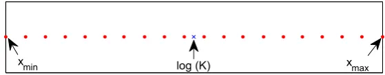
A good method for placing interpolation points can determine the accuracy of our scheme. To achieve this goal, we set a range of [xmin, xmax] and create N interpolation points via EMS (23). We then distribute the first N/2 points uni-formly in [xmin,log(K)], whereK is the strike price, and the remaining points in [log(K), xmax]. Our scheme for distributing the interpolation points is illustrated in Figure 1.

(10)

x_min _{log (K)} x_max

Figure 1. Uniform distributions of the interpolation points around the strike price obtained using EMS. The red dots represent the interpolation points. The blue cross is the location of the logarithmic strike price.

of interest as follows:

ˆ

xi ∈[ˆxmin,xˆmax] := [ log(K/20),log(2K) ]. (38) Based on this region, we can test the accuracy of our cubic spline interpolation scheme using a set of evaluation points ˆx∆_i x. We determine the grid points

ˆ

xi := ˆx∆i x= ˆxmin+j∆ˆx, j= 0,1,2, . . . , Neval−1 (39) where ∆ˆx = (ˆxmax−xˆmax)/Neval with xmin ≤ xˆmin ≤ xˆmax ≤ xmax and Neval is the number of evaluation points chosen. We will use the following three different measures for the errors: the maximum error

E∞= max

0≤i≤Neval

|f(ˆxi)−eu(ˆxi)|, (40)

the root-mean-square (rms) error

E2=

s

1 Neval

X

0≤i≤Neval

|V(exˆi_{, t)}−

e

u(ˆxi)|2, (41)

and the relative error

Erel.(ˆx, t) =

|V(exˆ, t)−_eu(ˆx, t)|

V(eˆx_{, t)} , (42)

where V(eˆx, t) and eu(ˆx, t) are the exact and approximate values at point (ˆx, t),

respectively.

We also calculate the rate of convergence of the maximum error and rms error usingE∞(ˆxi, T) andE2(ˆxi, T). We define the following formulae:

E∞(ˆxi, T) =C(1/N)R∞ (43)

for the maximum error and

E2(ˆxi, T) =C(1/N)R2 (44)

for the rms error, whereN is the number of interpolation points, C is a constant andR2 is the rate of convergence, which is linear when it equals one and quadratic when it equals two.

[image:10.595.137.417.49.104.2]

(11)

sensitivity or the rate of change in the option price _eu with respect to the change in the underlying logarithmic price and gamma Γ, the rate of change in delta with respect to the change in the underlying price. For4at any time τ, we have

4= ∂u(x, τ)e

∂x

ˆ

x

=

N

X

j=1 ρj(τ)

∂φ(|x−xj|)

∂x

ˆ

x

(45)

and for Γ, we have

Γ =∂u(x, τ)e

∂x

ˆ

x

=

N

X

j=1 ρj(τ)

∂2φ(|x−xj|)

∂x2

ˆ

x

. (46)

As discussed in Section 3, the explicit forms of∂φ(|x−xj|)/∂xand∂2φ(|x−xj|)/∂x2

are equal to (21) and (22), respectively.

The analytical price of a European call/put option in the Merton jump-diffusion model [44] is given by

VMJ(St, τ, K, r, q, σ)

=

∞

X

k=0

e−λ(1+η)τ((λ(1 +η)τ)k

k! VBS(St, τ, K, rk, σk, q), (47)

whereτ =T−t is the time to maturity,η =eµJ+ σ2_J

2 −1 represents the expected

percentage change in the stock price originating from a jump,σ_k2 =σ2+kσJ2

T−t is the

observed volatility,rk =r−λη+klog(1 +η)/(T−t), q is the dividend and VBS

the Black-Scholes price of a call and put computed as

VBS(St, τ, K, rk, σk, q)

=

Ste−qτΦ(d+,k)−Ke−rkτΦ(d−,k) call option,

Ke−rkτ_Φ(−d

−,k)−Ste−qτΦ(−d+,k) put option,

,

where Φ(·) is the cumulative normal distribution and

d+,k = log(St/K)+(rk −q+σ2

k/2)τ

σk

√

τ , d−,k =d+,k−σk

√ τ .

For the derivation ofVMJ(St, τ, K, r, q, σ), we refer the reader to [16, 44].

In general, for models in which the characteristic function of the L´evy process is known, an analytical solution for the PIDE (10) may be found using Fourier analysis [12, 38]. For the sake of simplicity and accuracy, we propose the Fourier space time-stepping method of Jacksonet al. rather than that of Carr-Madan [12] or the FFT method of Lewis [38]. The idea of this method is based on a Fourier transform of the PIDE. Using an FFT and inverse fast Fourier transform (FFT−1_), the European option price can be obtained. The pricing formula for evaluating the European option can be expressed as follows:

(12)

as

−σ 2_z2

2 +izγc+λ pα1 α1−iz

+ (1−p)α2 α2+iz

−1,

and VKou(S, T) is the payoff function (11). For more details on this method, we refer the reader to [31]. This method reportedly has a second-order convergence in space in the European cases.

Our RBF algorithm for numerically solving (10) with initial condition (11) is as follows:

(1) Find the RBF approximation to the initial valueu(x,0) using the ESM (see (23)) to obtain a set of interpolation pointsx1, . . . , xnand an initial vector

ρ ρ

ρ(0) = ρ1(0), . . . , ρN(0)

.

(2) Then, use ρρρ(0) as the initial value for the system (37). By using any stiff ODE solver, we can determineρρρ(T) at timeT.

(3) Finally, substituteρρρ(T) back into PN

j=1ρj(T)φ(|x−xj|) to obtain an ap-proximate value for u(x, T).

In our numerical experiment, we implement the algorithm in MATLAB R2007b and, as we did above, set our maximum and minimum logarithmic prices xmin

log(Smin)

and xmax log(Smax)

to−10 and 10, respectively. To obtain a more accurate approximation of the integral in (29), we set in both (25) and (27) to 3.72×10−40_{to determine a finite computational interval [y}

−, y]. Moreover, we use

the functionquadgk, which implements an adaptive Gauss-Kronrod quadrature for computing equation (30) and the functionode15s, which implements second-order backward differentiation formulas (BDFs) to calculate equation (37). The principal reason for choosing it is that according to [30], first- and second-order BDFs are A-stable (the stability region includes the entire left half of the complex plane). Because (37) is stiff, according to Theorem 4.11 (The Dahlquist second barrier) [30], the highest order of an A-stable multistep method,1 such as BDFs, is two.

All tabulated parameters except those in Tables 3, 6 and 9 are chosen from different reports in the literature. The parameter σ = 1 in Tables 3, 6 and 9 is selected to stress our numerical algorithm. From Table 1 to 9,E∞andE2 decrease when the number of interpolation pointsN increases. Our cubic spline interpolation scheme can obtain second-order convergence in space due to the limited smoothness of the cubic spline, which has second-order convergence (cf. [53]). In Figures 2, 3 and 4, oscillations do not occur around the strikeK for small values ofT when we approximate ∆ and Γ.In Table 10, we compare the results of the FD used by Briani et al. [9] with those using our cubic spline interpolation scheme. Our numerical approximation scheme can achieve lowerErel.(logS, T) values than either the

ARS-233 or Explicit scheme. Tables 10 and 12 provide additional comparisons between the accuracy of our cubic spline approximation scheme and that of Almendral and Oosterlee’s FDM and FEM with BDF2. To illustrate a fair comparison, we set our maximum and minimum logarithmic prices xmin and xmax to match those proposed by Almendral and Oosterlee in their numerical experiments. Thus, we set [xmin xmax] to [-4 4] and [-6 6] in the Merton model (Table 11) and Kou model (Table 12), respectively. Our cubic spline interpolation scheme can attain a lower Erel.(logS, T) value than the FDM or FEM with BDF2 in both the Merton and

Kou cases.

1_{Multistep methods are used to the numerically solve ordinary differential equations. Conceptually, a}

(13)

[image:13.595.175.383.97.192.2]

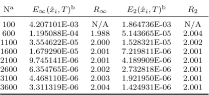
Table 1. E∞ andE2of the cubic spline interpolation for

pricing a European put under the Black-Scholes model. The parameters are as follows:r= 0.04, q= 0, σ= 0.29, K= 1 andT = 1.The parameters are taken from the literature [26]. The order of convergence is 2 in space.

Na _E_∞(ˆ_x

i, T)b R∞ E2(ˆxi, T)b R2

100 4.207101E-03 N/A 1.864736E-03 N/A 600 1.195088E-04 1.988 5.143665E-05 2.004 1100 3.554622E-05 2.000 1.528321E-05 2.002 1600 1.679290E-05 2.001 7.219811E-06 2.001 2100 9.745141E-06 2.001 4.189909E-06 2.001 2600 6.354765E-06 2.002 2.732818E-06 2.001 3100 4.468110E-06 2.003 1.921950E-06 2.001 3600 3.311319E-06 2.004 1.424931E-06 2.001

a _N _{is the number of interpolation points. ˆ}_x

i = logSi

[image:13.595.175.383.288.383.2]

is any evaluation point ranging fromS = 0.05 to 2, of which there are 1950.b_T _{is the maturity time.}

pricing a European put under the Black-Scholes model. The parameters are as follows:r= 0.05, q= 0, σ= 0.2, K= 1 andT= 2.The parameters are taken from the literature [?

]. The order of convergence is 2 in space. Na _E_∞(ˆ_x

i = logSi

pricing a European put under the Black-Scholes model. The parameters are as follows:r= 0.3, q= 0.1, σ= 1, K= 1 andT = 0.25, whereas the parameterσ= 1 is selected to stress our numerical algorithm. The order of convergence is 2 in space.

Na _E_∞(ˆ_x

100 2.325676E-03 0.000 1.404611E-03 N/A 600 6.473617E-05 1.999 3.856043E-05 2.007 1100 1.923322E-05 2.002 1.145625E-05 2.002 1600 9.079037E-06 2.003 5.411921E-06 2.001 2100 5.265272E-06 2.004 3.140776E-06 2.001 2600 3.430306E-06 2.006 2.048580E-06 2.001 3100 2.406208E-06 2.016 1.441039E-06 2.000 3600 1.782442E-06 2.007 1.068202E-06 2.002

i = logSi

[image:13.595.175.383.488.583.2]

(14)

[image:14.595.174.383.106.201.2]

pricing a European call under the Merton model. The pa-rameters are as follows: r = 0.05, q = 0, σ = 0.15, σJ= 0.45, µJ=−0.9, λ= 0.1, K= 1 andT = 0.25.The parameters are taken from [6]. The order of convergence is 2 in space.

Na _E_∞(ˆ_x

i = logSi

[image:14.595.174.383.305.401.2]

pricing a European put under the Merton jump-diffusion model. The parameters are as follows:r= 0.05, q= 0.02, σ = 0.15, σJ = 0.4, µJ = −1.08, λ = 0.1, K = 1 and

T = 0.1.The parameters are taken from [6]. The order of convergence is 2 in space.

Na _E_∞(ˆ_x

i = logSi

pricing a European call under the Merton model. The pa-rameters are as follows:r= 0.05, q= 0.01, σ= 1, σJ= 0.6,

µJ =−1.08, λ= 0.1, K = 1 andT = 1, whereas the pa-rameterσ= 1 is selected to stress our numerical algorithm. The order of convergence is 2 in space.

Na _E_∞(ˆ_x

i = logSi

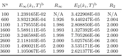
[image:14.595.175.382.504.600.2]

(15)

[image:15.595.175.385.106.201.2]

pricing a European put under the Kou model. The parame-ters are as follows:r= 0, q= 0, σ= 0.2, α1= 3, α2= 2,

λ= 0.2, p= 0.5, K= 1 andT = 0.2.The parameters are taken from the literature [2]. The order of convergence is 2 in space.

Na _E_∞(ˆ_x

i = logSi

[image:15.595.175.383.305.401.2]

pricing a European call under the Kou model. The parame-ters are as follows:r= 0.05, q= 0, σ= 0.15, α1= 3.0465,

α2= 3.0465, λ= 0.1, p= 0.3445, K= 1 andT= 0.25.The

parameters are taken from the literature [14]. The order of convergence is 2 in space.

Na _E_∞(ˆ_x

i = logSi

pricing a European put under the Kou model. The param-eters are as follows:r = 0.04, q = 0.03, σ= 1, α1 = 4,

α2= 4, λ= 0.3, p= 0.6K= 1 andT= 1,whereas the

pa-rameterσ= 1 is selected to stress our numerical algorithm. The order of convergence is 2 in space.

Na _E_∞(ˆ_x

i = logSi

[image:15.595.174.383.504.600.2]

(16)

0 0.5 1 1.5 2 −1

−0.8 −0.6 −0.4 −0.2 0

S

Δ

0 0.5 1 1.5 2 0

0.5 1 1.5

S

Γ

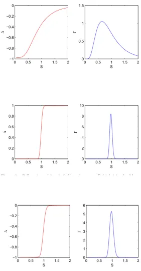
Figure 2. Put option delta ∆ (Left) and gamma Γ (Right) in the Black-Scholes Model. The number of interpolation points is 3600 . The number of evaluation points ranging fromS= 0.05 to 2 is 1950. The input parameters are provided in the caption for Table 3.

0 0.5 1 1.5 2 0

0.2 0.4 0.6 0.8 1

S

Δ

0 0.5 1 1.5 2 0

2 4 6 8 10

S

Γ

Figure 3. Call options delta ∆ (left) and gamma Γ (right) in the Merton model. The number of interpolation points is 3600. The number of evaluation points ranging fromS= 0.05 to 2 is 1950. The input parameters are provided in the caption for Table 5.

0 0.5 1 1.5 2 −1

−0.8 −0.6 −0.4 −0.2 0

S

Δ

0 0.5 1 1.5 2 0

1 2 3 4 5 6

S

Γ

[image:16.595.135.417.45.585.2]

(17)

[image:17.595.142.416.107.222.2]

Table 10. Comparison between the explicit scheme ([9]), ARS-233 scheme ([9]) and cubic spline interpolation scheme for evaluating European call/put options under the Merton jump-diffusion model. The input parameters are as follows:

r= 0.05, q= 0, σ= 0.2, σJ = 0.8, µJ= 0, λ= 0.1, K = 100, T = 1,and

x= log 100. The reference prices of 13.218501 (call) and 8.341444 (put) and the parameters are from [9].

Explicit scheme ARS-233 scheme N V alue Erel.(logS, T) V alue Erel.(logS, T)

Call 1024 13.286915 5.175624E-03 13.287427 5.214358E-03 Put 1024 8.319940 2.57797E-03 8.326102 1.839249E-03

Cubic spline N/A

N V alue Erel.(logS, T) V alue Erel.(logS, T)

[image:17.595.142.415.297.381.2]

Call 1024 13.219358 6.489263E-05 N/A N/A Put 1024 8.342301 1.027679E-04 N/A N/A Table 11. Comparison of the FDM with BDF2 ([2]), the FEM with BDF2 ([2]) and the cubic spline interpolation scheme for evaluating a European call (put) under the Merton model. The input parameters are as follows:r= 0, q= 0, σ= 0.2, σJ= 0.5, µJ= 0, λ= 0.1, K= 1, T= 1,andS= 1. The reference prices of 0.094135525 for both the call and put, and the parameters are from [2].

FD with BDF2 FE with BDF2 N V alue Erel.(logS, T) V alue Erel.(logS, T)

1025 9.411968E-02 1.682457e-04 9.412972E-02 6.165536E-05

Cubic spline N/A

1025 9.413023E-02 5.621522E-005 N/A N/A Table 12. Comparison of the FDM with BDF2 ([2]), the FEM with BDF2 ([2]) and the cubic spline interpolation scheme for evaluating a European call (put) under the Kou model. The input parameters are as follows:r= 0, q= 0, σ = 0.2, α1 = 3, α2 = 2, λ= 0.2, p= 0.5, K = 1, T = 0.2,and

S= 1. The reference prices of 0.0426761 for both the call and put, and the parameters are from [2].

FD with BDF2 FE with BDF2 N V alue Erel.(logS, T) V alue Erel.(logS, T)

513 4.240E-02 6.346096E-03 4.24579E-02 5.1285862E-03

Cubic Spline N/A

[image:17.595.143.414.455.539.2]

(18)

4.2 American Vanilla Put Options

In this section, we adapt an RBF algorithm to compute American put option prices. We then compare the option prices obtained from our RBF algorithm with those obtained from the Jackson et al. FST methods [31]. As mentioned in Section 2, an American put option problem is a free-boundary problem because of the possibility of early exercise at any point during its lifetime, leading to the free-boundary condition

u(x, τ) = max K−ex, u(x, τ).

Together with the smooth pasting condition mentioned in Section 2, this uniquely determines the exercise boundary.

The Jackson et al. FST methods suggest that their solutions can achieve second order in space when they implement their methods to price American put options. The methods are implemented in the context of the LCP. As described in Section 2, the value of an American option u(τ, x) is always greater than or equal to the payoff function G(ex). To numerically maintain the condition u(τ, x)−G(ex) ≥ 0 continuously (see Section 2), the boundary conditions must be applied. The numerical algorithm for this idea can be defined as follows:

V(S,(m+ 1)∆t, K, r, σ, q)

= max{FFT−1[ FFT [V(S, m∆t, K, r, σ, q) ]eψ∆t], G(ex),} (49) where the time interval ∆tis obtained by dividing the time to maturity T by the total numberM;m∆ is the time step, wherem∈ {0,1,2, . . . , M −1},ψ(z) is the characteristic function of the Merton/Kou models,V(S,(m+ 1)∆t, K, r, σ, q) is the American put price at time (m+ 1)∆t and the payoff condition G(ex) is equal to max(K −ex,0).These methods are also required to switch between the real and Fourier spaces at each time step when the American option prices are calculated for each time interval because no convenient representation exists for the max(., .) operator in Fourier space. For the full schematic and numerical description of this method, we refer the readers to [31].

As before, we use the ESM to approximateu(x,0) = max(K−ex_,_{0) and continue}

to work with the interpolation points found atτ = 0. The algorithm now reads as follows:

(1) Divide time to maturityT by the total number of time-stepsM to obtain time interval ∆tand create a list of equally spaced time-points m∆t,m∈ {0,1,2, . . . , M−1}.

(2) Find the RBF approximation for the initial value u(x,0) using the ESM. This will yield a set of interpolation points x1, . . . , xn, together with an

initial vectorρρρ(0) = ρ1(0), . . . , ρN(0)

.

(3) Assume that we have already determinedρρρ(m∆t) (ifm= 0, we knowρρρ(0)) in equation (37). Solve the system of (stiff) ODEs to findρρρ (m+ 1)∆t

at the next successive time step, (m+ 1)∆t.

(4) Then, at time (m+ 1)∆t, for each interpolation point xi, define

u xi,(m+ 1)∆t

= max (K−exi_),

N

X

j=1

ρj (m+ 1)∆t

φ(|xi−xj|)

.

(5) Find a new vectorρρρ (m+1)∆tsuch thatu xi,(m+1)∆t

=PN

(19)

1)∆tφ(|xi−xj|) for all i.

(6) Repeat Steps 3 to 5 until m=M −1. (7) Finally, substituteρρρ(T) back into PN

j=1ρj(T)φ(|x−xj|) to obtain an

ap-proximate value for u(x, T).

The settings of our numerical experiment are identical to those in Section 4.1. The results from Tables 13 to 18 suggest that our cubic spline interpolation scheme for pricing American put options is second order in spatial variables and first order in time variables when the number of interpolation numbers N and the number of time-steps M0 are twofold and fourfold, respectively. Moreover, Figures 5 to 7 indicate that oscillations do not occur around the strikeK for small or large values ofT when we approximate ∆ and Γ.

5. Conclusion

We implemented an RBF interpolation scheme to price American put and Euro-pean call/put options using the jump-diffusion model. By utilising the numerical scheme of Brianiet al., we determined a finite computational range for the global integral of the PIDE. Our results suggest that the interpolation scheme can achieve second-order convergence in both spatial variables for computing European prices. Our other numerical results demonstrate that our scheme is also able to obtain second-order convergence in spatial variables and first-order convergence in time variables when pricing American put options. In addition, we compared our in-terpolation scheme against the FDM and FEM. Our results suggest that one can achieve a high level of accuracy by implementing our method. For the RBF inter-polation, we used a cubic spline basis function rather than an MQ basis function. This basis function not only avoids the open question of choosing an optimal shape parameter for MQ but also avoids directly inverting an ill-conditioned cubic spline interpolant. Finally, throughout the analysis of both ∆ and Γ, our RBF interpo-lation method can resolve the oscilinterpo-lation problem around the strike in both the American and European cases.

(20)

[image:20.595.161.399.96.165.2]

Table 13. E∞andE2of the cubic spline interpolation for pricing

an American put under the Merton model. The parameters are as follows:r= 0.05, q= 0, σ= 0.15, σJ= 0.45, µJ=−0.9, λ= 0.1,

K= 1 andT= 0.25.The parameters are taken from [6]. The order of convergence is 2 in space and 1 in time.

Na _M

0b E∞(ˆxi, T)c R∞ E2(ˆxi, T)c R2

225 10 2.368536E-03 N/A 1.007946E-03 N/A 450 40 7.746936E-04 1.612 2.740154E-04 1.879 900 160 2.260415E-04 1.777 6.969946E-05 1.975 1800 640 6.362341E-05 1.829 1.888980E-05 1.884 3600 2560 1.613907E-05 1.979 4.715908E-06 2.002

i = logSi is any

evaluation point ranging fromS= 0.05 to 2, of which there are 1950.b M0 is the number of time steps .c T is the maturity

[image:20.595.161.398.268.336.2]

time.

Table 14. E∞andE2of the cubic spline interpolation for pricing

an American put under the Merton model. The parameters are as follows: r = 0.05, q = 0.02, σ = 0.15, σJ = 0.4, µJ = −1.08,

λ= 0.1, K = 1 andT = 0.1.The parameters are taken from the literature [6]. The order of convergence is 2 in space and 1 in time.

Na _M

225 10 3.401417E-03 N/A 7.995993E-04 N/A 450 40 1.318325E-03 1.367 2.451148E-04 1.706 900 160 3.744579E-04 1.816 6.873071E-05 1.834 1800 640 1.055849E-04 1.826 1.927219E-05 1.834 3600 2560 2.823205E-05 1.903 5.121082E-06 1.912

i = logSi is any

evaluation point ranging fromS= 0.05 to 2, of which there are 1950.b_M

0is the number of time steps.cT is the maturity time.

Table 15. E∞andE2of the cubic spline interpolation for pricing an

American put under the Merton model. The parameters are as follows:

r= 0.05, q= 0.01, σ= 1, σJ = 0.6, µJ =−1.08, λ= 0.1, K = 1 andT = 1,whereas the parameter σ = 1 is selected to stress our numerical algorithm. The order of convergence is 2 in space and 1 in time.

Na _M

225 10 4.935878E-03 N/A 1.613323E-03 N/A 450 40 1.236617E-03 1.997 3.725615E-04 2.114 900 160 3.093198E-04 1.999 9.101657E-05 2.033 1800 640 7.734030E-05 2.000 2.133679E-05 2.093 3600 2560 1.932168E-005 2.001 5.074520E-06 2.072

i = logSi is any

evaluation point ranging fromS = 0.05 to 2, of which there are 1950.b_M

[image:20.595.159.399.446.515.2]

(21)

[image:21.595.161.399.96.165.2]

American put under the Kou model. The parameters are as follows:

r= 0, q= 0, σ= 0.2, α1= 3, α2= 2, λ= 0.2, p= 0.5, K= 1 and

T= 0.2.The parameters are taken from the literature [2]. The order of convergence is 2 in space and 1 in time.

Na _M

225 10 1.508321E-03 N/A 5.589125E-04 N/A 450 40 7.233939E-04 1.060 1.759571E-04 1.667 900 160 1.958968E-04 1.885 4.733738E-05 1.894 1800 640 5.243753E-05 1.901 1.271703E-05 1.896 3600 2560 1.374207E-05 1.932 3.405083E-06 1.901

i = logSi is any

[image:21.595.161.398.268.336.2]

evaluation point ranging fromS= 0.05 to 2, of which there are 1950.bM0is the number of time steps.cT is the maturity time.

r = 0.05, q = 0, σ = 0.15, α1 = 3.0465, α2 = 3.0465, λ = 0.1,

p= 0.3445, K = 1 andT = 0.25.The parameters are taken from [14]. The order of convergence is 2 in space and 1 in time.

Na _M

225 10 1.933354E-03 N/A 8.983577E-04 N/A 450 40 8.487095E-04 1.188 2.783005E-04 1.691 900 160 2.497213E-04 1.765 7.257535E-05 1.939 1800 640 6.843085E-05 1.868 1.933309E-05 1.908 3600 2560 1.827216E-05 1.905 5.119491E-06 1.917

i = logSi is any

0is the number of time steps.cT is the maturity time.

r= 0.04, q= 0.03, σ= 1, α1= 4, α2= 4, λ= 0.3, p= 0.6, K= 1

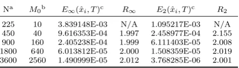
andT = 1,whereas the parameterσ= 1 is selected to stress our numerical algorithm. The order of convergence is 2 in space and 1 in time.

Na _M

225 10 3.839148E-03 N/A 1.095217E-03 N/A 450 40 9.616353E-04 1.997 2.458977E-04 2.155 900 160 2.405238E-04 1.999 6.111403E-05 2.008 1800 640 6.013812E-05 2.000 1.508359E-05 2.019 3600 2560 1.490999E-05 2.012 3.768285E-06 2.001

i = logSi is any

[image:21.595.161.398.447.515.2]

(22)

0 0.5 1 1.5 2 −1

−0.8 −0.6 −0.4 −0.2 0

S

Δ

0 0.5 1 1.5 2 0

1 2 3 4 5 6 7

S

Γ

Figure 5. Put option delta ∆ (left) and gamma Γ (right) in the Merton model. The number of interpolation points N is 1800, and the number of time stepsM0is 640. The number of evaluation points ranging fromS= 0.05

to 2 is 1950. The input parameters are provided in the caption for Table 13.

0 0.5 1 1.5 2 −1

−0.8 −0.6 −0.4 −0.2 0

S

Δ

0 0.5 1 1.5 2 0

1 2 3 4 5 6 7

S

Γ

Figure 6. Put option delta ∆ (left) and gamma Γ (right)in the Kou model. The number of interpolation pointsNis 1800, and the number of time steps

M0 is 640. The number of evaluation points ranging fromS = 0.05 to 2 is

1950. The input parameters are provided in the caption for Table 17.

0 0.5 1 1.5 2 −1

−0.8 −0.6 −0.4 −0.2 0

S

Δ

0 0.5 1 1.5 2 0

0.5 1 1.5 2 2.5

S

Γ

Figure 7. Put option delta ∆ (left) and gamma Γ (right)in the Kou model. The number of interpolation pointsNis 1800, and the number of time steps

M0 is 640. The number of evaluation points ranging fromS = 0.05 to 2 is

[image:22.595.136.417.47.586.2]

(23)

Appendix A. A Finite Computational Range in the Jump-diffusion Model

In the Merton model, suppose that a domain Ω ∈ _R for the European option priceu(x, τ) satisfies the Lipchitz inequality such that

|u(x₁, τ)−u(x2, τ)| ≤L|x1−x2|, ∀x1, x2 ∈Ω.

Then, we choose a parameter > 0 and select the bounded intervals [y−, y] as

the set of all pointsy that verify

k(y) = √ 1 2πσJ

e−

(y−_µJ)2 2σ2

J ≥.

Given the symmetry ofk(y), we sety−=−y. Then, the truncation of the integral

domain yielding an error in the approximation of the problem can be estimated by

Z ∞ −∞

(u(x+y)−u(x))k(y) dy−

Z y

−y

(u(x+y)−u(x))k(y) dy

≤L Z ∞ −∞

(x+y−x)k(y) dy−

Z y

−y

(x+y−x)k(y) dy

(A1a) ≤L Z −y −∞

|y|k(y) dy+

Z ∞ y |y|k(y) dy (A1b) = 2 Z ∞ y

y√ 1 2πσJ

exp(−(y−µJ) 2

2σ_J2 ) dy (A1c)

= 2

Z ∞

y−µJ

(y+µJ)

1 √

2πσJ

exp(− y 2

2σ_J2) dy (A1d)

= 2

Z ∞

y−µJ

(y+µJ)

1 √ 2πσJ exp(− y 2 2σ2 J

) dy (A1e)

≤2

Z ∞

y−µJ

(y+y)√ 1 2πσJ

exp(− y 2

2σ_J2) dy (A1f)

= √4σJ

2πexp(−

(y−µJ)2

2σ2_J ) (A1g)

= 2σ_J2. (A1h)

Thus, by using (A1g) and (A1h),

y =

q

−2σ2

Jlog(σJ

√

2π/2) +µJ (A2)

. We use the aforementioned arguments to determine the finite computational range [y−, y] in the Kou model. We carry out the reasoning for the positive semi-axis

(the reasoning is similar to that for the negative semi-axis) and setk(y) =pα1e−α1y fory ≥0 (1−p)α2eα2x fory < 0

(24)

equations:

Z ∞

0

(u(x+y)−u(x))λf(y) dy−

Z y

0

(u(x+y)−u(x))λf(y) dy

≤L

Z ∞

0

(x+y−x)λf(y) dy−

Z y

0

(x+y−x)λf(y) dy

(A3a)

≤L

Z ∞

y

|y|f(y) dy (A3b)

=

Z ∞

y

|y|pα1e−α1ydy (A3c)

=pα1e−yα1

1 α2₁ +

y

α1

(A3d)

[27, equation 3.351] = p

α1

e−yα1_{(1 +}_y

α1) (A3e)

≤ p α1

e−yα1_α

1ey (A3f)

=pey(1−α1) _(A3g)

=, (A3h)

resulting in

y= log(/p)/(1−α1). (A4)

Similar arguments can be applied toy <0. Thus,

y− =−log /(1−p)/(1−α2). (A5)

References

[1] A. Almendra,Numerical valuation of American options under the CGMY process, inExotic Option Pricing and Advanced L´evy Models, W. Schoutens, A. Kyprianou, and P. Wilmott, eds., Wiley, UK, 2004.

[2] A. Almendral and C. Oosterlee,Numerical valuation of options with jumps in the underlying, Applied Numerical Mathematics 53 (2005), pp. 1 – 18.

[3] A. Almendral and C.W. Oosterlee,On American options under the Variance Gamma process, Tech. rep., Delft University of Technology, 2004, to appear in Applied Mathematical Finance (not yet available).

[4] ———,Highly accurate evaluation of European and American options under the Variance Gamma process, Journal of Computational Finance 10 (2006), pp. 21–42.

[5] ———, Accurate evaluation of European and American options under the CGMY process, SIAM Journal on Scientific Computing 29 (2007), pp. 93–117.

[6] L. Andersen and J. Andreasen, Jump-diffusion processes: Volalitility smile fitting and numerical methods for option pricing, Review of Derivatives Research 4 (2000), pp. 231 – 262.

[7] L. Bos and K. Salkauskas,On the matrix[|xi−xj|3]and the cubic spline continuity equations, Journal

of Approximation Theory 51 (1987), pp. 81 – 88.

[8] S.I. Boyarchenko and S.Z. Levendorski˘i,Non-Gaussian Merton-Black-Scholes Theory,Advanced Se-ries on Statistical Science & Applied Probability, vol. 9, World Scientific Publishing Co. Inc., River Edge, NJ (2002).

[9] M. Briani, R. Natalini, and G. Russo,Implicit-explict numerical schemes for Jump-diffusion processes, Calcolo 44 (2007), pp. 33 – 57.

(25)

[11] R. Brummelhuis and R.T. Chan,An RBF scheme for option pricing in exponential l´evy models, Tech. rep., Birkbeck, University of London, 2011, sumitted to Journal of Applied Mathematical Finance. [12] P. Carr and D.B. Madan,Option valuation using the Fast Fourier Transform, Journal of

Computa-tional Finance 2 (1999), pp. 61–73.

[13] P. Carr, D.B. Madan, and E.C. Chang,The Variance Gamma process and option pricing, European Finance Review 2 (1998), pp. 79–105.

[14] P. Carr and A. Mayo,On the numerical evaluation of option prices in Jump Diffusion processes, The European Journal of Finance 13 (2007), pp. 353 – 372.

[15] P. Carr, H. Geman, D.B. Madan, and M. Yor,The fine structure of asset returns: An empirical investigation, Journal of Business 75 (2002), pp. 305–332.

[16] R. Cont and P. Tankov,Financial Modelling With Jump Processes, Chapman & Hall/CRC Financial Mathematics Series, Chapman & Hall/CRC, Boca Raton, Fla., London (2004).

[17] R. Cont and E. Voltchkova, A finite difference scheme for option pricing in jump diffusion and exponential L´evy models, SIAM Journal on Numerical Analysis 43 (2005), pp. 1596 – 1626.

[18] Y. d’Halluin, P. Forsyth, and K. Vetzalz,Robust numerical methods for contingent claims under Jump Duffusion process, IMA J. Num. Anal. 25 (2005), pp. 87 – 112.

[19] Y. d’Halluin, P.A. Forsyth, and G. Labahn,A penalty method for American options with Jump Diffusion processes, Numerische Mathematik 97 (2004), pp. 321 – 352.

[20] T. Driscoll and B. Fornberg, Interpolation in the limit of increasingly flat radial basis functions, Comput. Math. Appl. 43 (2002), pp. 413 – 422.

[21] G.E. Fasshauer, Meshfree Approximation Methods with MATLAB,Interdisciplinary Mathematical Sciences, vol. 6, World Scientific Sciences, Hackensack, N.J. (2007).

[22] G.E. Fasshauer and M.J. Mccourt,Stable evaluation of gaussian rbf interpolants (2010), http:// citeseerx.ist.psu.edu/viewdoc/summary?doi=10.1.1.188.7442.

[23] G.E. Fausshauer, A.Q.M. Khaliq, and D.A. Voss, inProceedings of A Parallel Time Stepping Approach Using Meshfree Approximations for Pricing Options with Non-smooth Payoffs, July, Third World Congress of the Bachelier Finance Society, Chicago, 2004.

[24] ———,Using meshfree approximation for multi-asset American option problems, J. Chinese Institute Engineers 27 (2004), pp. 563 – 571.

[25] B. Fornberg and G. Wright, Stable computation of multiquadric interpolants for all values of the shape parameter, Comput. Math. Appl. 47 (2004), pp. 497–523.

[26] M. Giles and R. Carter, Convergence analysis of Crank-Nicolson and Rannacher time-marching, Journal of Computational Finance 9 (2006), pp. 89–112.

[27] I.S. Gradshteyn and I. Ryzhik,Table of Integrals, Series, and Products, 5th ed., Academic Press, Inc., London (1994).

[28] A. Hirsa and D.B. Madan,Pricing American options under Variance Gamma, Journal of Computa-tional Finance 7 (2004).

[29] Y.C. Hon and X.Z. Mao,A radial basis function method for solving options pricing model, Financial Engineering 8 (1999), pp. 31–49.

[30] A. Iserles,A First Course in the Numerical Analysis of Differential Equations, Cambridge Texts in Applied Mathematics (2009).

[31] K.R. Jackson, J. Sebastian, and S. Vladimir,Fourier space time-stepping for option pricing with L´evy models, the Journal of Computational Finance 12 (2008), pp. 1–29.

[32] E.J. Kansa,Multiquadrics - a scattered data approximation scheme with applications to computational fluid dynamics - i.surface approximations and partial derivatives estimates, Comput. Math. Appl. 19 (1990), pp. 127–145.

[33] ———,Multiquadricsa scattered data approximation scheme with applications to computation fluid dynamics: Ii. solution to parabolic, hyperbolic and elliptic partial differential equations, Comput. Math. Appl. 19 (1990), pp. 147–161.

[34] S.G. Kou,A jump diffusion model for option pricing, Management Science 48 (2002), pp. 1086–1101. [35] S.G. Kou and H. Wang,Option pricing under a double exponential jump diffusion model, Tech. rep.,

Columbia University, 2001, working paper.

[36] E. Larsson, K. ˚Ahlander, and A. Hall,Multi-dimensional option pricing using radial basis functions and the Generalized Fourier Transform, Journal of Computational and Applied Mathematics 222 (2008), pp. 175–192.

[37] E. Larsson and B. Fornberg,Theorectical and computational aspects of multivariate interpolation with increasingly flat radial basis functions, Comput. Math. Appl. 49 (2005), pp. 103 – 130. [38] A.L. Lewis,A simple option formula for general Jump-diffusion and other exponential L´evy processes

(2001),http://www.optioncity.net/pubs/ExpLevy.pdf.

[39] L. Ling and E. Kansa,Preconditioning for radial basis functions with domain decomposition methods, Math. and Compt. Modelling 40 (2004), pp. 1413–1427.

[40] ———,A least-squares preconditioner for radial basis functions collocation methods, Adv. in Comput. Math 23 (2005), pp. 31–54.

[41] D.B. Madan and F. Milne,Option pricing with V. G. martingale components, Mathematical Finance 1 (1991), pp. 39–55.

[42] A.M. Matache, P.A. Nitsche, and C. Schwab,Wavelet galerkin pricing of American options on L´evy driven assets, 2003. working paper.

[43] A.M. Matache, C. Schwab, and T.P. Wihler,Fast numerical solution of parabolic integrodifferential equations with applications in finance, SIAM Journal on Scientific Computing 27 (2005), pp. 369–393. [44] R.C. Merton,Option pricing when underlying stock returns are discontinuous., Journal of Financial

Economics 3 (1976), pp. 125–144.

[45] U. Pettersson, E. Larsson, G. Marcusson, and J. Persson,Improved radial basis function methods for multi-dimensional option pricing, Journal of Computational and Applied Mathematics 222 (2008), pp. 82–93.

(26)

Math. Optim. 35 (1997), pp. 125 – 144.

[47] K.I. Sato,L´evy Processes and Infinitely Divisible Distributions, Cambridge University Press, Cam-bridge, U.K., New York (1999).

[48] W. Schoutens,L´evy Processes in Finance : Pricing Financial Derivatives, Wiley Series in Probability and Mathematical Statistics, Chichester : Wiley (2003).

[49] ———,Exotic options under L´evy models: An overview, Journal of Computational and Applied Mathematics 189 (2006), pp. 526 – 538.

[50] L.F. Shampine,Vectorized adaptive quadrature in matlab, Journal of Computational and Applied Mathematics 211 (2008), pp. 131 – 140.

[51] P. Tankov and E. Voltchkova,Jump-diffusion models: A practitioners guide(2009),http://people. math.jussieu.fr/~tankov/tankov_voltchkova.pdf.

[52] I.R. Wang, J.W.L. Wan, and P.A. Forsyth,Robust numerical valuation of European and American options under the CGMY process, Journal of Computational Finance 10 (2007), pp. 31–69. [53] H. Wendland,Scattered Data Approximation,,Cambridge Monographs on Applied and Computational