The PGST DBSCAN Algorithm for Mining Clusters from Massive Spatial temporal Data

2017 2nd _{International Conference on Artificial Intelligence and Engineering Applications (AIEA 2017)}

ISBN: 978-1-60595-485-1

The PGST-DBSCAN Algorithm for Mining Clusters

from Massive Spatial-temporal Data

YULIN YANG, LIANGDE LI, JINGCHI TANG and XIAOLI RAO

ABSTRACT

Below is a set of instructions for preparing your paper in a format suitable for the intended media for these proceedings. It is most important that you follow these guidelines as closely as possible and adhere to the margins (discussed below) for overall consistency and format relationship to all other papers in the intended proceedings. Print or type text as close to the margins as possible without going beyond these margins.

KEYWORDS

PGST DBSCAN, massive spatial-temporal data, Grid

INTRODUCTION

In recent years, with the development of location-acquisition technologies [1] such as GPS, sensor networks, and mobile devices and so on, massive spatial-temporal data are acquired. Spatial-temporal data mining, as a method of mining high-dimensional spatial-temporal data, has attracted increasing attention.

Spatial-temporal clustering analysis, as an important research area in spatial-temporal data mining, is of great significance to the identification of hotpot region or sparse region. K-means [2] is generally an efficient clustering method, but this algorithm requires the initialization of the cluster center and the number of clusters. For spatial-temporal clustering, it becomes impossible to identify the number of clusters and the cluster center in massive spatial-temporal data. The DBSCAN algorithm (Density-based spatial clustering algorithm)[3], (Density-based on the distance between spatial data points, efficiently achieves the discovery of clusters with arbitrary shape and the neglection of isolated points. In 2007, to achieve of the processing of spatial-temporal data, Birant[4-5] extended DBSCAN to ST-DBSCAN, which applied DBSCAN to three-dimensional spatial-temporal coordinate system instead of two-dimensional spatial coordinate system. However, ST-DBSCAN requires the calculation of the distance between data

_________________________________________

Yulin Yang, Jingchi Tang, Bell Honors School, The Nanjing University of Posts and Telecommunications, Nanjing, 210046, China. [email protected]

Liangde Li School of Electronic Science and Engineering, the Nanjing University of Posts and Telecommunications, Nanjing, 210046, China. [email protected]

points, resulting in long execution time and high memory consumption [6-7]. To achieve the efficiency of the processing of massive spatial-temporal data, GN-DBSCAN [8-9](Grid Based GN-DBSCAN) is proposed by Huang Ming in 2009, which divides the space into limited number of grid cells. GN-DBSCAN aims at the clustering of grid cells instead of data points. This paper firstly proposes GST-DBSCAN (Grid based temporal DBSCAN), which realize the grid quantization of spatial-temporal space, and the clustering of grid cells on spatial-spatial-temporal space.

Although GST-DBSCAN efficiently promotes the reduction of algorithm time complexity, a parallel implementation scheme of GST-DBSCAN on mass spatial-temporal data is of great significance, which is still a challenge. To overcome it, this paper further extends DBSCAN above to PDBSCAN (parallel GST-DBSCAN), which achieves the parallel implementation of GST-DBSCAN in the MapReduce environment of Hadoop.

The rest of the paper is organized as follows. Section 2 introduces the GST-DBSCAN, the input parameters are defined and the algorithm time complexity is analyzed in this section. Section 3 extends GST-DBSCAN to PGST-DBSCAN, the implementation schemes of Map phase and Reduce phase are discussed in this section. In Section 4, two comparison experiments are designed to compare the execution efficiency between GST-DBSCAN and DBSCAN, the execution efficiency between PGST-DBSCAN and GST-DBSCAN. The other experiment is introduced to explore the effect of input parameters on the clustering results. Overall conclusions are given in section 5.

GST-DBSCAN ALGORITHM

Definition of input parameters

Relevant definition of input parameters of GST-DBSCAN see as follows.

Definition1 ( ): , consists of 1 and 2, describes the scale of the grid cell. Among them, 1 is the length of the grid on the latitude and longitude axis, 2 is the length of the grid on the time axis.

Definition2 (core grid cell): If the number of points within a grid is greater than , then the grid is the core grid.

Definition3 (non-core grid cell): If the number of points within a grid is less than , then the grid is not the core grid.

Definition4 (adjacent grid cell): In the spatial-temporal coordinate system. If the two grid cells share the same surface, they are adjacent to each other.

The determination of and

In many cases [3], a simple heuristic is demonstrated to be effective to determine , which suggests that ln , where is the size of the data points. After the determination of , 1 can be calculated by the average point density, which can be given by the following equation:

1 ∙

Description of GST-DBSCAN

GST-DBSCAN clustering algorithm can be divided into two stages. The first stage is the allocation of data points into grid cells, the second stage is the process of merging the adjacent core grid cells.

Stage1: The construction of grid cells

Dividing the spatial-temporal coordinate system into grid cells. Traversing the dataset, every data point is allocated to corresponding grid cell according to its longitude, latitude and time component. The pseudo-code of this stage is shown as Algorithm1(Table.1).

The number of data points within each grid cell is counted. Marking the grid cells as core grid cell.

within which the number of points is greater than . The pseudo-code of this stage is shown as Algorithm(Table.2).

Table 1. Allocating data points to cells algorithm.

Algorithm 1: Allocating data points to cells algorithm

Input: The dataset of data points

Output: The set of cell<x, y, t>

The function allocate_to_cell( ) is to calculate which cell data[i] belongs to

For i =0 to n

<x,y,t>=allocate_to_cell(data[i].longitude ,data[i].latitude,data[i].time) cell<x, y, t>.numberofpoint+=1

End For

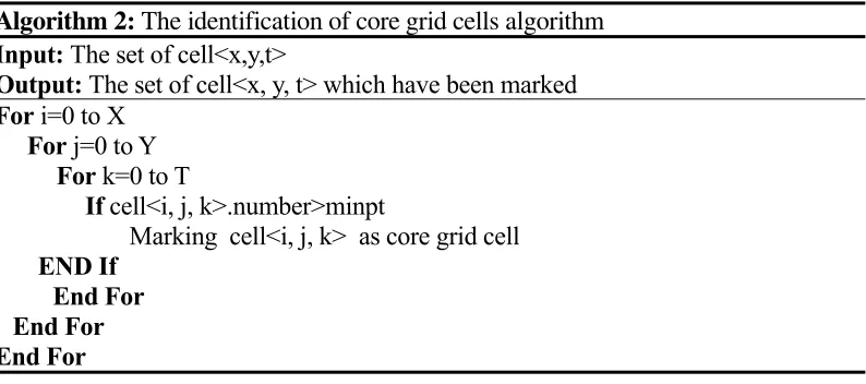
Table 2. The identification of core grid cells algorithm. Algorithm 2: The identification of core grid cells algorithm Input: The set of cell<x,y,t>

Output: The set of cell<x, y, t> which have been marked

For i=0 to X

For j=0 to Y

For k=0 to T

If cell<i, j, k>.number>minpt

Marking cell<i, j, k> as core grid cell END If

End For End For End For

Stage2: The process of merging

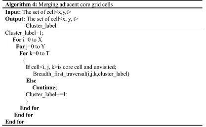
For the next unvisited core grid cell, repeating the process above. The algorithm ends until all the core grid cells have been visited. The pseudo-code of this stage is shown as Algorithm4(Table.4).

Table 3. Breadth first traversal algorithm.

Algorithm 3: Breadth_first_traversal algorithm Input: The set of cell<x,y,t>

Output: A cluster

Queue p

p.push(cell<i,j,k>)

While p! =null

Cell<x,y,t>=p.getfront() Cell<x, y, t> is visited

If the neighbor cell of cell<x,y,t> is core cell and unvisited p.push (neighbor cell of cell<x,y,t>)

END If

p.pop()

END While

Table 4. Merging adjacent core grid cells algorithm.

Algorithm 4: Merging adjacent core grid cells

Input: The set of cell<x,y,t>

Output: The set of cell<x, y, t> Cluster_label

Cluster_label=1;

For i=0 to X

For j=0 to Y

For k=0 to T {

If cell<i, j, k>is core cell and unvisited; Breadth_first_traversal(i,j,k,cluster_label)

Else

Continue;

Cluster_label+=1; }

End for End for End for

The analysis of time complexity

The time complexity of DBSCAN

find the time spent in the neighborhood of eps ), The best time complexity is o nlogn , The worst case complexity is o , n is the number of all points in the data set. In the second stage, the original DBSCAN clustering algorithm concatenates the core points within the . And connected core points of each group form a cluster. The average time complexity of this phase is o nlogn .

The time complexity of GST-DBSCAN

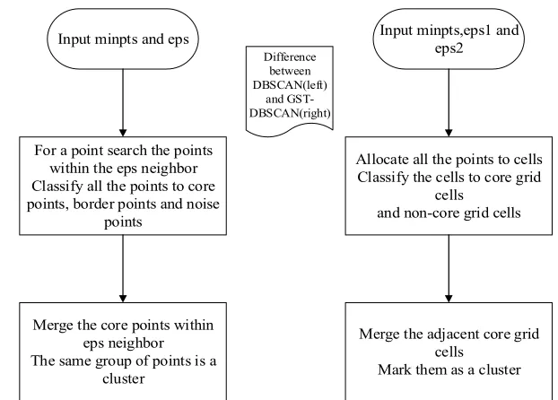
Input minpts and eps

For a point search the points within the eps neighbor Classify all the points to core points, border points and noise

points

Merge the core points within eps neighbor The same group of points is a

cluster

Input minpts,eps1 and eps2

Allocate all the points to cells Classify the cells to core grid

cells and non-core grid cells

Merge the adjacent core grid cells

Mark them as a cluster Difference

between DBSCAN(left)

and GST-DBSCAN(right)

Figure 1. The comparison of the two stages between GST-DBSCAN and original DBSCAN.

GST-DBSCAN firstly divides the spatial-temporal coordinate system into limited number of grid cells. Then the set of data points is traversed, each data points are classified into the corresponding grid cell and count the number of points within each grid cell is counted. If the number of points within the grid cells reach a certain threshold, the points in the grid are regarded as the core points. Those grid cells within which the number of points reach are considered as core grid cells. The time complexity of this stage is o n o c , where n is the number of data points, and c is the number of grid cells.

In the second stage. The improved GST-DBSCAN algorithm is to use the grid as the object. Breadth-first traversal strategy is adopted to merge the adjacent core grid cells. The time complexity o n o c .

In short, the best time complexity of the original DBSCAN algorithm is o nlogn , the average time complexity of GST-DBSCAN algorithm is o n o c . c is mainly affected by the scale of the target area and the partitioned grid cells, is irrelevant to the scale of the set of data points. The detailed comparison of the two stages between GST-DBSCAN and original GST-DBSCAN is shown as Fig.1.

PGST-DBSCAN ALGORITHM

The MapReduce parallelization of first stage

1) The Implementation of Map function

The spatial-temporal data is stored as text file. Each record of the spatial-temporal data can be written as <id, (lon, lat, t)>, where id is the id number of each record, lon, lat and t respectively represent longitude, latitude and time.

The task of the Map function is to allocate every spatial-temporal data point to its corresponding grid cells. The input Key-Value pairs of the Map function is Key=id , Value=cell(lon,lat,t). Each Map function reads a spatial-temporal data records. Which grid cell each data point belongs to is computed and grid cell (x, y, t) is generated. The result of Map function is output in the form of Key-Value pairs. The pseudo-code of Map function is shown as Table.5.

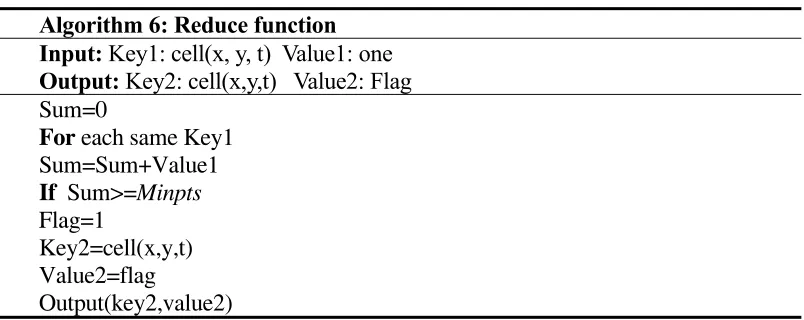
2) The Implementation of Reduce function

In order to mark core grid cells, it is necessary to determine whether the number of data points in each grid cell is greater than Minpts. Reduce function is required to count the number of data points of the same key, so as to mark the core grid. The pseudo-code of Map function is shown as Table.6.

Table 5. The pseudo-code of Map function.

Algorithm 5: Map function

Input: Key1: id Value1:cell(lon,lat,t)

Output: Key2: cell(x, y, t) Value2: one y = (lon - LON_MIN) / eps1

x =( lat - LAT_MIN) / eps1

time = Time / eps2

Cell cell = new Cell(x, y, time) Key2=cell(x,y,t)

Value2=one

Output(Key2,Value2)

Table 6. The pseudo-code of Reduce function.

Algorithm 6: Reduce function Input: Key1: cell(x, y, t) Value1:one

Output: Key2:cell(x,y,t) Value2: Flag Sum=0

For each same Key1

Sum=Sum+Value1

If Sum>=Minpts

Flag=1

Key2=cell(x,y,t) Value2=flag

The MapReduce parallelization of second stage

1) The Implementation of Map function

The Map function in the second stage is required to read the output text file of Reduce function in the second stage, achieve the format conversion.

2) The Implementation of Reduce function

Reduce function in the second stage is required to read the output of the Map function, the breadth of the first traversal strategy is adopted to visit the non-visited grid cells. Output is the form of Key-Value pairs, key is the grid cell, value is the grid cell corresponding Cluster Label. The pseudo-code of Reduce function is shown as Table.7.

EXPERIMENT

Experiment A is designed to prove GST-DBSCAN performs better than DBSCAN in execution time. Experiment B compares the performance between PGST-DBSCAN and GST-DBSCAN without MapReduce Environment. Experiment C explores the effect on which the change of input paraments of PGST-DBSCAN has. To verify the effect of clustering, we implement the visualization of the clustering result.

Data Source

Our data source is the GPS trajectory dataset, which was collected in Geolife project[10-12](Microsoft Research Asia) by 182 user in a period of over three years (from April 2007 to August 2012). The size of the total original data is 1.7GB, it becomes 500MB after the data cleaning.

Table 7. The pseudo-code of Reduce function.

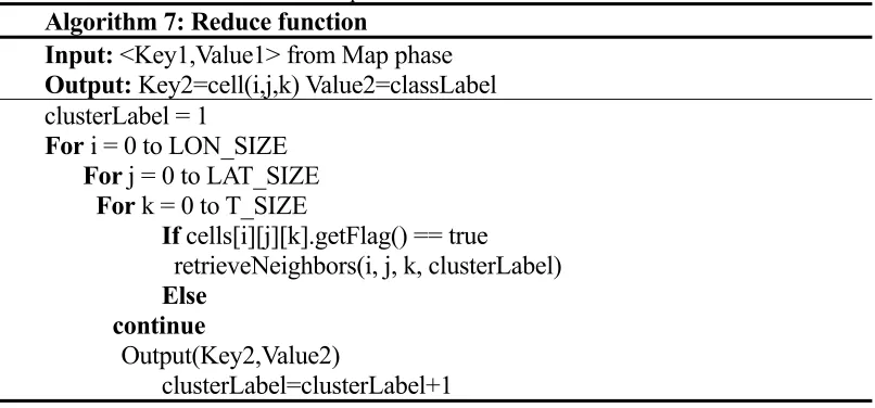
Algorithm 7: Reduce function

Input: <Key1,Value1> from Map phase

Output: Key2=cell(i,j,k) Value2=classLabel clusterLabel = 1

For i = 0 to LON_SIZE

For j = 0 to LAT_SIZE For k = 0 to T_SIZE

If cells[i][j][k].getFlag() == true

retrieveNeighbors(i, j, k, clusterLabel)

Else

continue

Output(Key2,Value2)

Experiment Environment

 Single-machine environment: The experiment environment is arranged with win10 operating system and eclipse integrated development environment.

 Cluster environment: The cluster environment is built in three physical hosts, Hadoop Framework is adopted, including a computer as name node, with memory for 8GB and CPU for i7-3770, the other other computers as data node, data node1 with memory for 8GB CPU for i7 -4790, data node2 memory with memory for 4GB and CPU for 2 core-E7200.

The comparison of execution time between GST-DBSCAN and DBSCAN

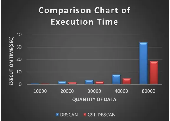
Java programming language is adopted to implement the GST-DBSCAN and DBSCAN algorithm to compare execution time between GST-DBSCAN and DBSCAN algorithm. With single-machine environment, the execution time of the two algorithms is measured at 10000,20000,30000,40000,80000 records, their values are shown as the Fig.2 below.

By analyzing the histogram above, we can conclude that:

When the amount of data points is small, GST-DBSCAN differs a little from DBSCAN in execution time.

With the amount of data points increasing, the execution time of DBSCAN grows faster than GST-DBSCAN.

The comparison between PGST-DBSCAN and GST-DBSCAN

Based on the MapReduce framework, we code the program of PGST-DBCAN, running the program on the Hadoop platform with three nodes. On the other hand, GST-DBSCAN is implemented in single-machine environment. The execution time of the two algorithms is measured at 14000,400000,24000000 records, their values are shown as the Table.7 below.

Figure 2. The comparison chart of execution time. 0

10 20 30 40

10000 20000 30000 40000 80000

EXECUTION 

TIME(SEC)

QUANTITY OF DATA

Comparison Chart of 

Execution Time

Table 7. The comparison of execution time between PGST-DBSCAN and GST-DBSCAN. Environment Data size Data records Execution time Clusters Number Single-machine 6.72M 14000 25s 1334 Single-machine 30M 400000 225s 1843 Single-machine 500M 24000000 out of memory

Cluster of multi-machine 6.7M 14000 100s 1334 Cluster of multi-machine 500M 24000000 197s 16654

By analyzing the table above, we can conclude that:

1) When the amount of data points is small, GST-DBSCAN with single-machine environment perform better than PGST-DBSCAN with distributed cluster environment. Compared to the cost of data operation, resource scheduling, task allocation, communication cost more execution time, which is the main reason why GST-DBSCAN perform better than PGST-GST-DBSCAN.

2) With the amount of data points increasing, the execution time of GST-DBSCAN grows far faster than PGST-DBSCAN.

3) When the amount of data points is large, the running process of GST-DBSCAN with single-machine environment may be out of memory, while PGST-DBSCAN with distributed cluster environment performs well.

The effect of input parameters to PGST-DBSCAN clustering algorithm

To explore the consequence that the input parameter, esp1, esp2, Minpts have on the result of clustering. We took Minpts for 8, eps1 for 0.0005, esp2 for 2 as the initial input parameters. In the experiment to determine the parameters, we have taken the initial experience minpt for 8, eps1 = 0.0005, for eps2, we have 2 hours for a time period, let eps2 = 2. After that, we modify the input parameters, Made a controlled trial. Here is our experimental table analysis.

The effect of esp1 and esp2 to PGST-DBSCAN clustering algorithm The clustering results vary with the input parameter esp1, shown as Table.8

By analyzing the table above, we can draw the conclusions that when esp1 becomes smaller, the number of grid cells becomes greater, the execution time of PGST-DBSCAN increases a little, while the number of clusters generated dramatic increases.

The effect of Minpts to PGST-DBSCAN clustering algorithm

The clustering results vary with the input parameter Minpts, shown as Table.9

Table 8. Clustering results with the change of esp1.

Data size Data records Cells number Execution time Cluster number 500M 24000000 500*400*12 193s+1.6s 6972 500M 24000000 800*640*12 196s+2.2s 12367 500M 24000000 1000*800*12 195s+2.5s 16654 500M 24000000 1200*800*12 245s+3.1s 20835 500M 24000000 2000*1600*12 246s+4.7s 41798 500M 24000000 5000*4000*12 282s+9.8s 65635

Table 9. Clustering results with the change of Minpts.

By analyzing the table above, we can draw the conclusions that when Minpts becomes smaller, the execution time of PGST-DBSCAN decreases a little, while the number of clusters generated dramatic decreases.

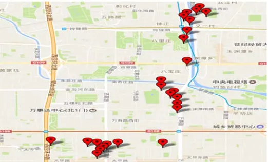
The visualization of Clustering results

Due to the number of clusters generated is too large, if all the clusters generated is shown in this paper, the observability will become worse. Based the consideration above, we divided the urban area of Beijing into 100 parts, and we took 2h as the time interval. One of them from 4:00 AM to 6:00 AM is shown as Fig.3, another one from 6:00 AM to 8:00 AM is shown as Fig.4. Each drop in the Fig.3 and Fig.4 represents a cluster, the average longitude and latitude of grid cells within each cluster are adopted to respectively represent the longitude and latitude of its corresponding drop.

By analyzing the clusters above, from 4:00 to 6:00 AM, the majority of the clusters are distributed in residential areas, the GPS users may be in the rest, from 6:00 to 8:00 AM, the majority of the clusters are distributed in road area and work area, the GPS users may be on the way to work.

Figure 3. One of the visualization of Clustering results from 4:00 AM to 6:00 AM.

CONCLUSION

Having conducted thorough experiment and analysis, we can make the conclusions as follows. Firstly, GST-DBSCAN algorithm we proposed achieves higher efficiency than DBSCAN. The comparison experiment we did have identified that the GST-DBSCAN algorithm speeds up the velocity of clustering. Secondly, the PGST-DBSCAN algorithm we proposed not only further speeds up the velocity of clustering, but also improves the processing ability for massive data. The result of comparison experiment also indicates that PGST-DBSCAN performs better than GST-DBSCAN for the reduction of clustering time and the processing ability for massive data. At last, an experiment is designed to explore the effect that the input parameters have on the clustering results, whose results show that the number of clusters generated has a positive correlation with esp1, a negative correlation with Minpts. For further studies, we can extract some meaningful features of spatial-temporal data to cluster with PGST-DBSCAN.

ACKNOWLEDGMENTS

This work is supported by the National Natural Science Foundation of P. R. China (No. 41571389,61472193), the Open Project of Key Laboratory of Spatial Data Mining & Information Sharing of Ministry of Education, Fuzhou University (No.2016LSDMIS07, the State University Student STITP of China (No. SZDG2016041).

REFERENCES

1. Wang M., Ji G., Zhao B., et al. A Parallel Clustering Algorithm Based on Grid Index for Spatio-temporal Trajectories [C]//Advanced Cloud and Big Data, 2015 Third International Conference on. IEEE, 2015: 319-326.

2. Jiang X., Li C., Xiang W., et al. Parallel implementing k-means clustering algorithm using MapReduce programming mode [J]. Huazhong Keji Daxue Xuebao(Ziran Kexue Ban)/ Journal of Huazhong University of Science and Technology(Nature Science Edition), 2011, 39.

3. Ester M., Kriegel H.P., Sander J., et al. A density-based algorithm for discovering clusters in large spatial databases with noise [C]//Kdd. 1996, 96(34): 226-231.

4. Birant D., Kut A. ST-DBSCAN: An algorithm for clustering spatial–temporal data [J]. Data & Knowledge Engineering, 2007, 60(1): 208-221.

5. Wang M., Wang A., Li A. Mining spatial-temporal clusters from geo-databases [J]. Advanced Data Mining and Applications, 2006: 263-270.

6. Sundararajan S., Karthikeyan S. A Study On Spatial Data Clustering Algorithms In Data Mining."[J]. 2013.

7. Parimala M., Lopez D., Senthilkumar N.C. A survey on density based clustering algorithms for mining large spatial databases [J]. International Journal of Advanced Science and Technology, 2011, 31(1): 59-66.

8. Wu B, Wilamowski B.M. A Fast Density and Grid Based Clustering Method for Data with Arbitrary Shapes and Noise [J]. IEEE Transactions on Industrial Informatics, 2016.

9. Huang M., Bian F. A grid and density based fast spatial clustering algorithm [C]//Artificial Intelligence and Computational Intelligence, 2009. AICI'09. International Conference on. IEEE, 2009, 4: 260-263.

11. Yu Zheng, Quannan Li, Yukun Chen, Xing Xie, Wei-Ying Ma. Understanding Mobility Based on GPS Data. In Proceedings of ACM conference on Ubiquitous Computing (UbiComp 2008), Seoul, Korea. ACM Press: 312-321.