1
A Level-Set Method for Convective-Diffusive Particle Deposition
Y.F. Yap1,*, F.M. Vargas2 and J.C. Chai1
1Depart. of Mechanical Eng., The Petroleum Institute, Abu Dhabi, UAE. 2Depart. of Chemical Eng., The Petroleum Institute, Abu Dhabi, UAE.
*Corresponding author:
Tel: +971 2 607 5175
Fax: +971 2 607 5200
Email address: [email protected]
Address:
The Petroleum Institute
Department of Mechanical Engineering
2 Abstract
This article presents a fixed-mesh approach to model convective-diffusive particle deposition onto surfaces. The deposition occurring at the depositing front is modeled as a first order reaction. The evolving depositing front is captured implicitly using the level-set method. Within the level-set formulation, the particle consumed during the deposition process is accounted for via a volumetric sink term in the species conservation equation for the particles. Fluid flow is modeled using the incompressible Navier-Stokes equations. The presented approach is implemented within the framework of a finite volume method. Validations are made against solutions of the total concentration approach for one- and two-dimensional depositions with and without convective effect. The presented approach is then employed to investigate deposition on single- and multi-tube arrays in a cross-flow configuration.
Keywords: level-set, deposition, first order reaction
1 Introduction
The phenomena of deposition, either benign or malign, are encountered in many engineering applications. Examples include but are not limited to thin film production in semiconductor wafer manufacturing, coatings for various surface-finishing purposes and fouling in heat exchangers and pipelines. For deposition to be enhanced, controlled or prevented, an in-depth understanding of deposition process is important. Such an understanding can be derived experimentally. For example, detailed physical insights on deposition of asphaltene particles in capillary tubes are obtained from lab-scale experimental investigations via quantification of the growing asphaltene deposit layer [1, 2]. However, for deposition processes involving small time and length scales, e.g. in thin film production and perhaps coatings, expansive high-resolution equipments are required to provide data with the time and length scales convincingly resolved. For fouling, the time scale can be large. Therefore, scaled experimental investigations are time consuming. Occasionally, extreme conditions, e.g. high pressure environment, and hazardous chemical materials are encountered. Experimental interrogations, if possible, then demand extreme cautiousness. In view of this,
theoretical investigations, in particular numerical simulations, play an essential complementary role in understanding various deposition processes. It provides useful detailed insights and the ability to predict these processes.
Central to all deposition processes is the dynamics of the evolving depositing front. Successful simulations of deposition processes require an accurate prediction of the moving depositing front. Based on the way the depositing front is handled, methods for predicting the movement of the depositing front can generally be categorized into two categories. These are the front-tracking and the front-capturing methods.
The movement of the depositing front is tracked explicitly in front-tracking methods. For example in the moving mesh method [3, 4], the boundary of the mesh is used to represent the depositing front. The mesh deforms during the deposition process so that the boundary of the mesh always coincides with the moving depositing front. This approach offers superior accuracy both for the location of the depositing front and imposition of related boundary conditions. However, when the deformation of the mesh is large, remeshing is required to maintain numerical stability. Remeshing is not straight forward in the presence of topological changes. Extension of a moving mesh
3
In front-capturing methods, the depositing front is no longer explicitly tracked but implicitly captured via an indicator function. As there is no explicit tracking required, a fixed-mesh can readily be used. Front-capturing methods include but are not limited to the total concentration approach, the VOF method and the level-set method. The total concentration approach [5, 6] was initially developed in the spirit of the enthalpy method [7, 8] for etching problems. The reacted concentration of the etchant, analogous to the latent heat content in the enthalpy method, captures the etch front implicitly. Recently, the total concentration approach was adapted to model
deposition process via a new definition of the total concentration [9]. In this approach, the depositing front is captured implicitly by the concentration of the deposit. The approach was demonstrated for deposition problems in one- and two-dimensions.
The VOF method [10] is often used to capture the interface between two immiscible fluids. In the work of [11, 12], the VOF method has been adapted to modeling deposition processes employed in semiconductor wafer manufacturing. The VOF method captures the depositing front implicitly via convection of the volume fraction of the reference phase by an underlying velocity field. During the calculation procedure, the depositing front must be reconstructed. This is one of the challenging aspects of employing the VOF method; particularly in three-dimensional problems.
In the level-set method [13], the deposition front is captured by the level-set function. Convection of the level-set function by the velocity of the depositing front captures implicitly the motion of the depositing front. Early attempts of applying the level-set method for deposition process were made for applications in the semiconductor industries [14-16]. In these pioneering works, if desired both deposition and etching can be accounted for within a unified framework. Demonstrations were made for cases where velocity of the depositing front is given in various explicit forms. The level-set method has the inherit advantages of automatic handling of topological changes and the ease of extension to three-dimensional problems.
Depending on the deposition process, there can be more than one type of particles involved. The term “particles” is used loosely in this article to refer to solid particles, ionic species or other to-be-deposited materials. For example, in modeling deposition of asphaltene onto the walls of petroleum wells or pipelines, only asphaltene particles, though of various sizes, need to be accounted for [17,18]. However, two types of particles, i.e. accelerator and cupric particles, are considered in a typical electrodeposition [19]. This is a more sophisticated deposition process where the accelerator particles, the cupric particles and the applied electric current interact to produce the copper deposit layer.
4
For small scale problem, a non-continuum treatment of particle transport, e.g. the molecular dynamic approach [1], is sometimes more desirable.
The deposition process occurring at the depositing front can either be of a physical or chemical origin. For example in a physical vapor deposition process, gas particles solidify on surfaces to form the deposit layer [27]. In a chemical vapor deposition process, gas particles react or
decompose on surfaces to produce the deposit layer [28]. The deposition flux at the deposition front has to be modeled based on these mechanisms. Varied though the types of mechanisms, the
condition at the depositing front frequently appears in the form of a generalized third type of boundary condition. Examples include asphaltene particle deposition (modeled as first order reaction) [17], SiO2 deposition [21] and copper electrodeposition [19, 23, 24]. Therefore, from a modeling point of view, the simplest first order reaction would be sufficiently representative of a general deposition process. It is worth pointing out that this boundary condition is incorporated as an additional volumetric particle sink localized at the depositing front [19, 24]. With this, the implementation of the boundary condition explicitly on a moving front is circumvented. To model particle deposition in Lagrangian particle transport approach, the concept of critical size and sticking probability [29] are often employed with where particles are probabilistically assumed deposited once their distance from the wall is less than the critical length. There are of course empirical models for specific type of particle deposition processes [30]. Applications of these empirical models need appropriate adaptation.
Interestingly and to the best knowledge of the authors, deposition process of a single species of particles modeled as a first order reaction under the framework of a level-set method has not been investigated. The present article intends to fill in this gap. This article presents a level-set method for deposition of a single species of particle onto surfaces. The deposition occurring at the
depositing front is modeled as a first order reaction. The particles are driven by convective-diffusive transport. The results obtained serve to understand the more complicated deposition processes.
The remaining of the article is divided into five sections. The deposition problem is described in Section 2. This problem is then formulated within the framework of the level-set method in Section 3. The solution procedure is given in Section 4. In Section 5, validations and results are presented and discussed. Finally, a few concluding remarks are given.
[image:4.595.57.263.553.660.2]2 Problem Descriptions
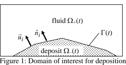
Figure 1: Domain of interest for deposition.
Figure 1 shows a schematic of the domain of interest . It consists of a fluid region and a deposit region , i.e.
t
t . These two regions are separated by the depositing front
t . Within the fluid region, there exists a suspension of solid particles. These particles gradually deposit onto the depositing front. As a result of the deposition, the depositing front evolves with a velocity of ui and the deposit region grows.
deposit –(t) fluid +(t)
(t)
i
nˆ
i
5 3 Mathematical Formulation
3.1 Capturing the Depositing Front
The depositing front is embedded into a level-set function [13], mathematically defined as
t x t x t x d d if if if , , 0 , (1)where d is the shortest distance from the depositing front. Under such a representation, the depositing front is given by 0. Convection of the level-set function under an appropriate velocity field captures implicitly the movement of the depositing front. This appropriate velocity field ui,ext is derived from ui (which is only available at the depositing front) by extending it off the depositing front with the following property maintained.
t x uui,ext i , (2)
The extension can be constructed in such a way that ui,ext is constant along the curve normal to the depositing front. This can be easily achieved using the approach suggested by [31] as
x n S t , 0 ˆ (3)where can be any component of ui,ext . In Eq. (3), the unit normal vector nˆ and the signum function S
are given respectively by
nˆ (4a)
0 if 0 if 0 if , 1 , 0 , 1 S (4b)With ui,ext properly constructed, the movement of the depositing front can then be captured as
x u
t iext
, 0 , (5)
To maintain as a distance function, i.e. 1, after the convection of via Eq. (5), is set to the steady-state solution of Eqs. (6) [32].
x sign t , 0 1 (6a)where t is a pseudo time for and sign
is given by [33] as
2 2 2 x sign (6b)and is subjected to the following initial condition.
x x ,0 (6c)
6
Figure 2: Deposition of particles onto
t in the control volume V.The deposition process is modeled as a first order reaction with the deposition flux expressed as
t x n C k uqDi D ˆi , (7)
where D, kD, C and nˆi are the density of the deposit, the deposition reaction rate, the particle concentration and unit normal vector pointing into the fluid region respectively. If the deposition process is instead modeled as a higher order reaction, Eq. (7) needs to be modified. However, the formulation outlined below can account for a higher order reaction easily by including some minor modifications. Rearrangement of Eq. (7) gives the velocity of the depositing front as
t x n C k u D i Di
, ˆ
(8)
Within the control volume (CV) V (Fig. 2), the rate of particle consumed during the deposition process at the depositing front can be evaluated as
V D h t D ht D i i
t i C dV C k d CdS k dS n n C k dS n q S 0 lim 0 ˆ ˆ ˆ (9)
where the Dirac delta function is defined as
otherwise 2 0 if , 0 , 2 / cos1
(10)
Note that Eq. (9) has been converted from a surface integral into a volume integral. Since there is no particle within the deposit region, the distribution of
used in the conversion has been shifted towards the fluid region following the approach of [34]. With this conversion, Eq. (9) can be employed to model the deposition process occurring at the depositing front via a localized volumetric particle sink concentrated around
t in the conservation equation governing the particle transport within the domain . This conservation equation can then be written as
x kC C D C u tC
,
(11)
where u and D are velocity of the fluid and diffusion coefficient respectively. The diffusion coefficient D can be expressed conveniently using as
0 if 0 if , , 0 D D (12)The last term in Eq. (11), derived in the spirit of Eq. (9), accounts for the particle consumed during the deposition process. In the solution of Eq. (11), the following initial and boundary conditions apply. Initial Condition fluid +(t) (t) dS nˆi
h deposit
–(t)
7
0 if 0 if , , 0 0 , x C x C o (13a) Boundary conditions
x t C
xC , B , x1 and t0 (13b)
x t n F
x CD B
, ˆ , x2 and t0 (13c)
where 12 and 12 .
During the movement of the depositing front via the convection of through Eq. (5), some of the particles in the immediate adjacence of the depositing front are trapped in the deposit region. If left untreated, the amount of trapped particles in the growing deposit region increases with time. To alleviate this problem, the trapped particles will be redistributed evenly to all other CVs of the fluid region. At the end of each time step, the amount of trapped particles is calculated as
C H V
Ctrapped 1 (14a)
where the Heaviside function H
is defined as
if if if , 1 , sin 2 1 2 , 0 H (14b)Then, for all the CVs of the fluid region, the following correction is made to C such that
V H C C C trapped (14c)To complete the procedure, the concentration of the particles C for all the CVs in the deposit region is set to C0.
3.3 Fluid Transport
The particles can be carried by a flowing fluid. To model the convection effect, the incompressible forms of the continuity and the Navier-Stokes equations are employed for the whole domain .
u 0 , x (15)
x u u p u u tu T
,
(16)
where and are the fluid density and viscosity respectively. The deposit is modeled as an extremely viscous fluid, i.e. a solid. This is easily achievable in the present formulation with the following definition of the viscosity.
0 if 0 if , , (17)For the velocity, the boundary condition can be a combination of (1) inlet velocity, (2) outflow boundary and (3) no slip.
4 Numerical Method
8
staggered velocity components are defined at the surface of the CVs. The combined convection-diffusion effect is modeled using the Power Law. A fully implicit scheme is used for time integration. The velocity-pressure coupling of the Navier-Stokes equations is handled with the SIMPLER algorithm.
To capture the evolving depositing front accurately, the level-set method requires higher order numerical schemes. The evolution of the level-set function (Eq. 5) and its redistancing (Eq. 6) are spatially discretized with WENO5 [37] and integrated using TVD-RK2 [38]. These schemes are computationally intensive. To reduce the computational effort, the level-set method is implemented in a narrow-band procedure [33] where the level-set function is solved only within a band of certain thickness from the interface. This reduces one order of computational effort.
4.1 Solution Algorithm
The overall solution procedure for the presented method can be summarized as follows: (1) Specify the initial conditions (i.e. t0) of u, p, and C.
(2) Advance the time step to tt.
(3) Solve Eqs. (15) and (16) for utt and ptt. (4) Solve Eq. (11) for
t t
C .
(5) Calculate ui tt from Eq. (8) and then
t t ext i
u
,
from Eqs. (3) and (4).
(6) Solve Eq. (5) for tt and perform redistancing using Eq. (6). (7) Repeat steps (3) to (6) until the solution converges.
(8) Perform particle redistribution via Eq. (14). (9) Repeat steps (2) to (8) for all time steps.
5 Results and Discussions
For the ease of discussions, the following dimensionless parameters are used in the remainder of the article. These are the dimensionless particle concentration, Peclet, Damkohler and Reynolds
numbers defined respectively as
D o o
C C
* (18)
D L u
Pe o (19)
D L k
DaD D (20)
uoL
Re (21)
where L and uo are the characteristic length and velocity respectively. The dimensionless time, coordinates and concentration are given respectively by
L t u
t* o (22)
L x
9 L
y
y* (23b)
D C C
* (24)
In the case when there is no fluid flow, the characteristic velocity is redefined as uoD/L and therefore the Peclet number reduces to Pe1.
5.1 Validations
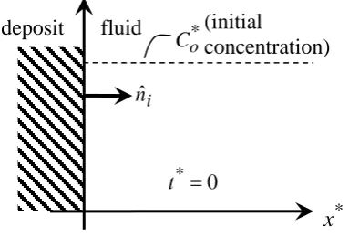
[image:9.595.56.248.616.746.2]5.1.1 Deposition in a One-Dimensional Semi-Infinite Domain
Figure 3a shows a schematic of a deposition process in a one-dimensional semi-infinite domain. At
0
*
t , the particle concentration in the fluid region is uniformly set to Co* and the depositing front is located at x* 0. As there is not fluid flow involved, diffusion is the sole mechanism of
transporting the particles. During the deposition process, particles are deposited onto the depositing
front resulting in the movement of the depositing front. For a given t*0, the depositing front is located at x** after an additional deposit layer of thickness * formed on the existing
depositing front. Since particles are consumed in the process, the particle concentration decreases. The initial and boundary conditions correspond to this problem are
Initial condition: *
*
o
C
C for 0x* (25a)
Boundary conditions:
0
*
x C
for x* 0 (25b)
* *
C
C for x* (25c)
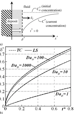
Figure 3b shows the effect of DaD on the thickness of the deposit layer. For these cases, the initial particle concentration is set to Co* 0.5. Although not shown here, these are grid independent solutions. To enforce the boundary condition of Eq. (25c), solutions were obtained for x*5 and 10. These solutions are identical. Therefore, x*5 is sufficient numerically to represent a semi-infinite domain. Generally, * grows faster with a larger DaD. Superimposed in the same figure are the solutions from [9] using the total concentration (TC) approach. The present solutions (LS) are in good agreement with those of [9].
i
nˆ Co
*
x deposit
(i) t*0
fluid *
o
10 (a)
[image:10.595.61.334.60.454.2](b)
Figure 3: One-dimensional deposition, (a) domain of interest and (b) effect of DaD with C* 0.5.
5.1.2 Deposition in a Two-Dimensional Square Enclosure
Figure 4a shows a two-dimensional square enclosure containing a uniform suspension of particles. Driven solely by diffusion, these particles deposit gradually on the four walls. Due to symmetry, the lower left quarter of the enclosure is modeled with the following initial and boundary conditions. Initial condition:
* *
o
C
C for 0x*1 and 0 y* 1 (26a)
Boundary conditions:
0
*
x C
for x* 0 ,1 (26b)
0
*
y C
for y*0 ,1 (26c)
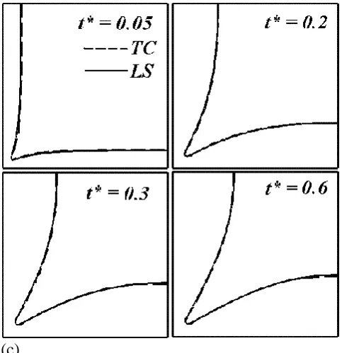
For this validation exercise, Co*0.5. Figures 4b and 4c show the solutions for the case of 1
D
Da and 10 respectively. The presented grid independent solution is obtained using a mesh of 160
160 CVs with t*5.0103. Superimposed onto these figures are the solutions obtained using the TC approach. The present predictions are in good agreement with those of the TC approach.
(ii) t* 0
*
i
nˆ Co fluid
deposit
*
x *
o
C
*
C (current concentration) (initial
11
During the deposition process, the particles in the regions near the corners of the enclosure are deposited to both the horizontal and vertical segments of the depositing front. More particles in these regions are consumed generally. Therefore, the concentration of the particle is generally lower in these regions. For the case of DaD 1, deposition is slow compared to diffusion. Diffusion is able to replenish the particles consumed at the depositing front near the corners of the enclosure. A more uniform particle distribution along the depositing front can then be achieved. As a result, the deposit layers on the walls grow more uniformly. However, for the case of DaD 10, deposition is much faster than diffusion. The particles consumed in the regions near the corners of the enclosure cannot be replenished in time by the sole mechanism of diffusion. The regions near the corners of the enclosure have comparatively much lower particle concentration. In fact the depositing front near the corners of the enclosure does not move much after the initial stage of the deposition process, forming a crevice-like feature near the corners of the enclosures.
(a)
(b)
*
o
C
*
x deposit
fluid *
y
2
12 (c)
Figure 4: Deposition in a two-dimensional square enclosure with Co*0.5, (a) domain of interest, (b) DaD 1 and (c) DaD 10.
5.1.3 Deposition in Two-Dimensional Channel with Flowing Fluid
A fluid carrying particles in the form of suspension flows into a two-dimensional channel as shown in Fig. 5a. The dimensionless length and height of the channel are 3 and 1 units. Initially, there is no deposit in the channel. As the fluid flows, the particles deposit onto the walls of the channel,
forming deposit layers. Since the deposit is impermeable, it changes the flow field. The flow field and the concentration field are therefore coupled together. Making use of the symmetry of the problem, solution was computed only for the lower half of the domain. In the definition of Re and
Pe, the characteristic length and characteristic velocity are the height of the channel and the inlet velocity respectively. The following initial and boundary conditions apply.
Initial conditions:
0
*
u , C*0 for 0x*3 and 0 y*0.5 (27a) Boundary conditions:
At the inlet (x*0)
1
*
u , v*0,
otherwise , 5 . 0 25 . 0 , 0 * * *
C y
C o (27b)
At the outlet (x*3) 0 * * x u
, v*0, 0
* * x C (27c)
At the wall (y* 0) 0
*
u , 0
* * y C (27d)
13 0
* *
y u
, v*0, 0
* *
y C
(27e)
The evolution of the depositing front for the case of Re1, Co* 0.1 Pe15 and DaD 10 predicted by the present approach is shown in Fig. 5b. This is the grid independent solution
obtained on a mesh of 24040CVs with t*5103. This case was also investigated by [9] and the solution is superimposed. The two solutions agree well with each other. The dimensionless
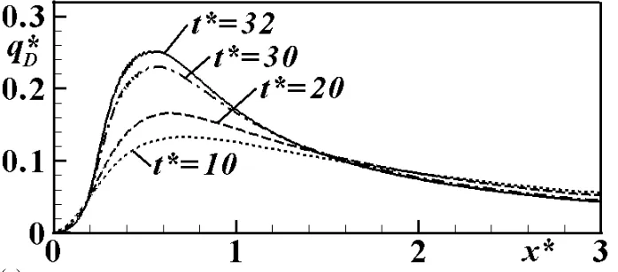
deposition flux (defined as q*D qD/(kDCo) where qD is the amount of deposit formed over a unit area of the wall) along the channel at different time is shown in Fig. 5c. Generally, q*D is much higher near the inlet as a result of a higher particle concentration. The deposit layer near the inlet grows faster and is therefore thickest. The concentration of the particle decreases downstream as particles are deposited along the flow. The thickness of the deposit layer then decreases along the channel.
(a)
(b)
deposit *
o
u
fluid 1
3
*
x *
14 (c)
Figure 5: Deposition on the walls of a two-dimensional channel with flowing fluid, (a) domain of interest, (b) evolution of the depositing front and (c) dimensionless deposition flux for Re1,
1 . 0
*
o
C Pe15 and DaD 10. 5.2 Case Studies
[image:14.595.60.340.357.467.2]5.2.1 Cross-Flow Deposition on a Single-Tube Array
Figure 6: Cross-flow deposition on a single-tube array.
Figure 6 shows a cross-flow through a single-tube array. The flowing fluid carries a suspension of particles. These particles gradually deposit onto the surface of the tubes. Deposit layers form on the surface of the tubes. Given the symmetries of the problem, only the region within the dotted box needs to be modeled. This portion of the figure is enlarged. The tube located at
0.75,0.5
has a radius of R0.2. The following initial and boundary conditions apply.Initial conditions:
0
*
u , C*0 for 0x*1.5 and 0 y*0.5 (28a) Boundary conditions:
At the inlet (x*0)
1
*
u , v*0, C*Co* (28b)
At the outlet (x*1.5) 0
* *
x u
, v*0, 0
* *
x C
(28c)
At the lower and upper symmetric boundaries (y*0,0.5) deposit fluid
0.5
*
x *
y 1.5
tubes
15 0
* *
y u
, v*0, 0
* *
y C
(28d)
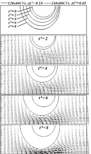
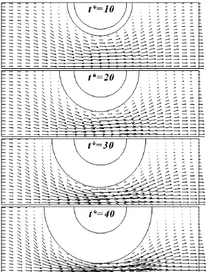
The evolution of the depositing front for the case of Re1, Co* 0.1, Pe15 and DaD 10 is shown in Fig. 7. Shown in the first plot of Fig. 7 is the depositing front at t* 0, 2, 4, 6 and 8 obtained from two different meshes, i.e. a mesh of 12040CVs with t*0.10 and a mesh of
80
240 CVs with t* 0.05. Examination of Fig. 7 clearly indicates that grid independent solution can be obtained on a mesh of 12040CVs with t*0.10. The evolution of both the depositing front and the corresponding flow field is sequentially shown in the remaining plots of Fig. 7. To avoid overcrowding the figure, not every velocity vector is plotted. Only one vector in every five in the x-direction and one in every two in the y-direction are plotted. The flowing fluid carries particles towards the frontal surface of the tube (inlet-facing). Given the rich particle
concentration and a high reaction rate (DaD 10), most of these particles deposit onto the frontal surface of the tube. Some of the remaining particles of course are carried by flow downstream along the surface of the tube and deposit onto the rear surface of the tube (outlet-facing). With this, it is expected that a much thinner deposit layer formed at the rear surface of the tube. The deposit layer
almost blocks the entire domain at t*8.
The evolution of the depositing front for a case of lower DaD is shown in Fig. 8. For this particular case of DaD 1, although the particle concentration at the frontal surface of the tube is high, most of these particles do not deposit because of the low reaction rate. Instead, these particles will remain there or be carried by the flowing fluid downstream. In fact, the reaction rate is so slow that
deposition is not much affected by the particle concentration. The deposition rate at the frontal and rear surfaces of the tube is almost identical. As a result, a deposit layer of almost uniform thickness formed around the tube.
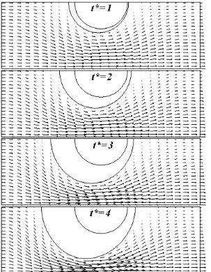
The effect of Pe can be investigated via a comparison of Figs. 7 and 9. In Fig. 9, Pe is lowered to 5 but withRe1, Co* 0.1 and DaD 10 maintained. A lower Pe suggests a stronger diffusion transport of the particles. After particles are consumed at the depositing front, the region near the depositing front would have a lower particle concentration. A concentration gradient is then
16
17
18
Figure 9: Deposition on single-tube array for the case of Re1, Co* 0.1, Pe5 and DaD 10. 5.2.2 Cross-Flow Deposition on a Multi-Tube Array
Figure 10: Cross-flow deposition on a multi-tube array.
A configuration similar to that of Fig. 6 but with a multi-tube array is considered. Depicted in Fig. 10 is the new staggered tube arrangement. There are now three tubes in each row. The tubes are labeled sequentially from A (upstream) to F (downstream). Tubes A, B, C, D, E and F are located respectively at
0.5,0.5
,
0.8,0
,
1.1,0.5
,
1.4,0
,
1.7,0.5
and
2.0,0
. The radii of these tubes are identical, i.e. R0.2. The initial and boundary conditions of Eq. (28) are enforced.fluid
0.5
*
x *
y
2.5
tube
*
x
B D F
[image:18.595.56.332.517.637.2]19
The first plot of Fig. 11 shows the grid independent test conducted for the case of Re1, Co* 0.1, 15
Pe and DaD 10. Judging from this plot, a mesh of 20040CVs with t* 0.10 is
sufficient to fully resolve the features of the solution. The depositing front is depicted together with the corresponding flow field in the remaining plots of Fig. 11. Again, the velocity vectors are selectively plotted to avoid overcrowding the figure. For all tubes, a thicker deposit layer formed on the frontal surface is generally observed. Among these tubes, the thickest deposit layer forms on tube A. This is expected as tube A nearest to the inlet where the flowing fluid carries with it the highest possible particle concentration. As particles deposit on tubes located along the streamwise direction, the particle concentration generally decreases along the streamwise direction. When the flowing fluid reaches tube F, it has the lowest particle concentration. Therefore, the thinnest deposit layer forms on tube F.
20
21
22
Figure 13: Deposition on multi-tube array for the case of Re1, Co* 0.1, Pe5 and DaD 10. 6 Conclusions
The present article presents a level-set approach for modeling convective-diffusive particle deposition processes. Deposition occurring at the depositing front is modeled as a first order reaction. The particle consumed during the deposition process is incorporated as a volumetric sink term in the species conservation equation. Fluid flow is modeled using the incompressible Navier-Stokes equations. The presented approach is implemented and validated against solutions of the total concentration approach. It was then used to investigate deposition on single- and multi-tube array in a cross-flow configuration.
Acknowledgement
This work was supported by The Petroleum Institute under Grant: RAGS-11008.
References
23
2. D. Broseta, M. Robin, T. Savvidis, C. Fejean, M. Durandeau and H. Zhou, Detection of Asphaltene Deposition by Capillary Flow Measurements, SPE/DOE Improved Oil Recovery Symposium, Apr. 3-5, 2000, Tulsa, Oklahoma.
3. Z. Zhu, K.W. Sand and P.J. Teevens, A numerical study of under-deposit pitting corrosion in sour petroleum pipelines, Northern Area Western Conference, Feb. 15-18, 2010, Calgary, Alberta.
4. Z. Chen and S. Liu, Simulation of Copper Electroplating Fill Process of Through Silicon Via, Packaging Technology 3 (2010) 433-437.
5. P. Rath, J.C. Chai, Y.C. Lam and V.M. Murukeshan, A total concentration fixed-grid method for two-dimensional wet chemical etching, J. Heat Transfer 129 (2007) 509-516.
6. P. Rath and J.C. Chai, Modelling convection-driven diffusion-controlled wet chemical etching using a total-concentration fixed-grid method, Num. Heat Transfer B 53 (2008) 143-159. 7. N. Shamsundar and E.M. Sparrow, Analysis of multidimensional conduction phase change via
the enthalpy model, J. of Heat Transfer 97 (1975) 333-340.
8. V.R. Voller, Numerical Methods for phase-change problem, Handbook of Numerical Heat Transfer 2nd ed., John Wiley & Sons Inc, Hoboken, New Jersey, 2006.
9. Q. Ge., Y.F. Yap, F.M. Vargas, M. Zhang and J.C. Chai, A Total Concentration Method for Modeling of Deposition, Numer. Heat Transfer, Part B 61 (2012) 311-328.
10. C.W. Hirt and B.D. Nichols, Volume of fluid (VOF) method for the dynamics of free boundaries, J. Comput. Phys. 39 (1981) 201-225.
11. J.J. Helmsen, Volume of fluids methods applied to etching and deposition, American Physical Society, Gaseous Electronics Conference 1996, Oct. 21-24.
12. J. Helmsen, E. Puckett, P. Colella, and M. Dorr, Two new methods for simulating photolithography development in 3D, Proc. SPIE 2726 (1996) 253-261.
13. S. Osher and J.A. Sethian, Fronts propagating with curvature-dependent speed: Algorithms based on Hamilton-Jacobi formulations, J. Comput. Phys. 79 (1988) 12.
14. D. Adalsteinsson and J.A. Sethian, A level-set approach to a unified model for etching,
deposition and lithography I: Algorithm and two-dimensional simulations, J. Comput. Phys. 120 (1995) 128-144.
15. D. Adalsteinsson and J.A. Sethian, A level-set approach to a unified model for etching,
deposition and lithography II: Three-dimensional simulations, J. Comput. Phys. 122 (1995) 348-366.
16. J.A. Sethian and D. Adalsteinsson, An Overview of Level Set Methods for Etching, Deposition, and Lithography Development, IEEE Trans. Semiconductor Manufacturing 10-1 (1997) 167-184.
17. F.M. Vargas, J.L. Creek and W.G. Chapman, On the Development of an Asphaltene Deposition Simulator, Energy Fuels 2010 (24) 2294-2299.
18. A.S. Kurup, F.M. Vargas, J. Wang, J. Buckley , J.L. Creek, Hariprasad, J. Subramani and W.G. Chapman, Development and Application of an Asphaltene Deposition Tool (ADEPT) for Well Bores, Energy & Fuels 25 (2011) 4506-4516.
19. D. Wheeler, D. Josell and T.P. Moffat, Modeling Superconformal Electrodeposition Using The Level Set Method, J. Electrochem. Soc. 150 (2003) C302-C310.
20. H.A. Al-Mohssen and N.G. Hadjiconstantinou, Arbitrary-pressure chemical vapor deposition modeling using direct simulation Monte Carlo with nonlinear surface chemistry, J. Comput. Phys. 198 (2004) 617-627.
24
22. C. Heitzinger, J. Fugger, O. Häberlen, and S. Selberherr, Simulation and Inverse Modeling of TEOS Deposition Processes Using a Fast Level Set Method, The 2002 Int. Conf. on Simulation of Semiconductor Processes and Devices, Sept. 4-6, Kobe, 191-194.
23. J.A. Sethian and Y. Shan, Solving partial differential equations on irregular domains with moving interfaces, with applications to superconformal electrodeposition in semiconductor manufacturing, J. Comput. Phys. 227 (2008) 6411-6447.
24. M. Hughes, N. Strussevitch, C. Bailey, K. McManus, J. Kaufmann, D. Flynn and M.P.Y. Desmulliez, Numerical algorithms for modelling electrodeposition: Tracking the deposition front under forced convection from megasonic agitation, Int. J. Numer. Methods Fluids 64 (2010) 237-268.
25. D. Eskin, J. Ratulowski, K. Akbarzadeh and S. Pan, Modelling asphaltene deposition in turbulent pipeline flows, The Canadian J. Chem. Eng. 89 (2011) 421-441.
26. A. Guha, Transport and Deposition of Particles in Turbulent and Laminar Flow, Annu. Rev. Fluid Mech. 40 (2008) 311-341.
27. D. M. Mattox, Handbook of Physical Vapor Deposition (PVD) Processing, Noyes Publications, New Jersey, 1998.
28. H.O. Pierson, Handbook of Chemical Vapor Deposition: Principles Technology and Applications, 2nd ed., Noyes Publications, New Jersey, 1999.
29. M. Abdolzadeh, M.A. Mehrabian and A.S. Goharrizi, Numerical study to predict the particle deposition under the influence of operating forces on a tilted surface in the turbulent flow, Adv. Powder Tech. 22 (2011) 405-415.
30. K.A. Lawal, V. Vesovic and E.S. Boek, Modeling Permeability Impairment in Porous Media due to Asphaltene Deposition under Dynamic Conditions, Energy & Fuels 25 (2011) 5647-5659. 31. S. Chen, B. Merriman, S. Osher, and P. Smereka, A simple level set method for solving Stefan
problems, J. Comput. Phys. 135 (1995) 8.
32. M. Sussman, P. Smereka, S. Osher, A level set approach for computing solution to incompressible two-phase flow, J. Comput. Phys. 114 (1994) 146-159.
33. D. Peng, B. Merriman, S. Osher, H. Zhao and M. Kang, A PDE-based fast local level-set method, J. Comput. Phys. 155 (1999) 410-438.
34. Y.F. Yap, J.C. Chai, T.N. Wong, N.T. Nguyen, K.C. Toh and H.Y. Zhang, Particle transport in microchannels, Numer. Heat Transfer, Part B 51 (2007) 141-157.
35. S.V. Patankar, Numerical Heat Transfer and Fluid Flow, Hemisphere Publisher, New York, 1980.
36. H.K. Versteeg and W. Malalasekera, An Introduction to Computational Fluid Dynamics: The Finite Volume Method, 2nd ed., Prentice Education Limited, England, 2007.
37. G.-S. Jiang and D. Peng, Weighted ENO schemes for Hamilton–Jacobi equations, SIAM J. Sci. Comput. 21 (2000) 2126-2143.
25 Nomenclature
C particle concentration *
C dimensionless particle concentration *
o
C dimensionless initial particle concentration
trapped
C amount of trapped particles in the deposit region d normal distance from the interface
dS elemental surface area dV elemental volume D diffusion coefficient
D
Da Damkoler number
h thickness of the CV in Fig. 2 H modified Heaviside function
D
k reaction rate for deposition L characteristic length nˆ unit normal vector
i
nˆ unit normal vector at the depositing front p pressure
Pe Peclet number q deposition flux
D
q deposition flux per unit wall area
o
u characteristic velocity
u velocity component in the x-direction *
u dimensionless velocity component in the x*-direction u fluid velocity
i
u velocity of the depositing front
ext i
u, velocity extended from ui x position vector
R radius of tube Re Reynolds number
sign Sign function S signum function
C
S rate of particle consumed during deposition
t time
t pseudo-time *
t dimensionless time
*
x , y* dimensionless Cartesian coordinate x, y Cartesian coordinate
v velocity component in y-direction *
v dimensionless velocity component in y*-direction V
control volume
modified Dirac delta function
*
26 component of ui,ext
viscosity of fluid density of fluid
D
density of the deposit depositing front domain of interest
fluid region
27 List of Figures
Figure 1: Domain of interest for deposition.
Figure 2: Deposition of particles onto
t in the control volume V.Figure 3: One-dimensional deposition, (a) domain of interest and (b) effect of DaD with C* 0.5. Figure 4: Deposition in a two-dimensional square enclosure with Co*0.5, (a) domain of interest,
(b) DaD 1 and (c) DaD 10.
Figure 5: Deposition on the walls of a two-dimensional channel with flowing fluid, (a) domain of interest, (b) evolution of the depositing front and (c) dimensionless deposition flux for
1
Re , * 0.1
o
C Pe15 and DaD 10. Figure 6: Cross-flow deposition on a single-tube array.
Figure 7: Deposition on single-tube array for the case of Re1, Co* 0.1, Pe15 and DaD 10. Figure 8: Deposition on single-tube array for the case of Re1, Co* 0.1, Pe15 and DaD 1. Figure 9: Deposition on single-tube array for the case of Re1, Co* 0.1, Pe5 and DaD 10. Figure 10: Cross-flow deposition on a multi-tube array.