A Novel Parameter Estimation Method of the Quadratic FM Signal in Alpha stable Distribution Environment

2017 2nd International Conference on Wireless Communication and Network Engineering (WCNE 2017) ISBN: 978-1-60595-531-5

A Novel Parameter Estimation Method of the Quadratic FM Signal in

Alpha-stable Distribution Environment

Li LI

1,*

and Xiao-fei SHI

2 1

Information Engineering College, Dalian University, Dalian 116622, China 2

Information Science and Technology College, Dalian Maritime University, Dalian 116026, China *Corresponding author

Keywords: Alpha-stable distribution, Fractional lower-order statistics, Fractional ambiguity function, Quadratic FM signal, Parameter estimation.

Abstract. This paper takes the Alpha-stable distribution as the noise model and studies the parameter estimation problem of quadratic FM signal in the impulsive noise environment. Since the conventional algorithms degenerate severely in the impulsive noise environment, this paper proposes a novel method of fractional ambiguity function basing on the fractional lower-order statistics (FLOS-FAF). Firstly, the fractional lower order Instantaneous correlation function is proposed and is performed by the fractional Fourier transform (FRFT). Secondly, parameters of quadratic FM signal are jointly estimated by peak searching the FLOS-FAF and dechirping method. Simulation experiments verify that the proposed algorithm can suppress the impulse noise and has good performance when poor SNR condition exists.

Introduction

The quadratic frequency modulated signal has been widely used in signal processing fields such as in the modern communication, sonar and radar systems and biomedical and so on. Due to the three dimensional (3D) motion characteristics of the target, the received signal often contains cubic term in its phase function. The polynomial phase signal has many modulated parameters, and can enhance difficulty of receiver estimation signal parameters and processing gain. Therefore, the polynomial phase signal is the common signal form in low probability of interception radar, such as broadband linear FM radar and nonlinear frequency modulation radar.

The optimum method to estimate the QFM signal is Maximum likelihood (ML) estimation. However, its computation complexity is extremely great and the global convergence is not always guaranteed. As a computationally efficient alternative, the high-order ambiguity function (HAF) and the Product high-order ambiguity function (PHAF) can estimate the Polynomial phase signal (PPS)'s parameters with P one-dimensional searches via multiple nonlinear operations on the received signal

[2-4]_{. Moreover, the Polynomial Wigner-Ville distribution (PWVD) is also a high-order multiple}

transform technique for dealing with PPS. In recent years, fractional Fourier transform (FRFT), has attracted increasingly more attention in signal processing and has been widely applied in detection, parameter estimation and direction of arrival estimation of the LFM signal [6-7].

Analysis of Fractional Ambiguity Function Basing the Fractional Lower Order Statistics

Fractional Ambiguity Function

Instantaneous autocorrelation function Rs

(

t,τ

)

of the signal s t( ) is defined by

(

,

)

(

2

) (

* 2

)

s

R t_{τ =}s t_+τ s t_{−τ (1)}

The fractional ambiguity function (FAF) of the signal s t( ) _{, namely the FRFT of Eq.1,}

(

, ,

)

FAF _ρ m_{τ can be written as}

(

, ,

)

s

(

,

)

(

,

)

FAF m R t K t m dt

ρ

ρ τ +∞ τ

−∞

=

∫

(2)

where _ρ is the rotation angle and m _{is the frequency in FRFT domain,} K

(

t m_,

)

ρ is the kernel function

of the fractional Fourier transform. K

(

t m,

)

ρ can be expressed as

(

)

(

)

(

)

(

)

(

)

(

)

2 2

1 cot exp cot 2 csc cot ,

, , 2

, 2 1

j j t mt m n

K t m t m n

t m n

ρ

ρ π ρ ρ ρ ρ π

δ ρ π

δ ρ π

 _{− − + ≠}

 

= − =



+ = +



(3)

The signal s t( ) _{with a cubic term in its phase function, also called Quadratic frequency modulated}

signal, is defined as

( )

0exp

(

2

(

0 1 2 2 3 3

)

)

s t ₌b j _π a ₊a t₊a t ₊a t ₍₄₎

where b0 is the signal amplitude, and a ii, =0,1, 2, 3 are signal phase factors, the amplitude and phase factors are real and unknown [8].

With the use of Eq.1, Instantaneous autocorrelation function of the signal Eq.4 can be expressed as

(

)

2

(

(

2 3

)

)

0 3 2 1 3

, exp 2 3 2 4

s

R t_{τ =}b j _π a_τt ₊ a_τt₊a_{τ +}a_{τ (5)}

For a given delayτ, Rs

(

t,τ

)

is a linear frequency modulation signal. According to the definition of

FRFT in [11], we can obtain the fractional ambiguity function (FAF) of the signal Eq.4, FAFs

(

α, ,mτ

)

can be written as

(

)

(

)

(

)

(

)

(

)

(

)

(

)

(

)

(

)

2 2 3

0 1 3

2

3 2

FAF , , , ,

exp π _{cot 2 2}

exp π _{6 cot 4 2 csc}

s u Rs t K t u dt

b A j u a a

j a t a u dt

ρ

ρ

ρ τ τ

ρ τ τ

τ ρ τ ρ

+∞ −∞

+∞ −∞

=

= + +

+ + −

∫

∫

i (6)

According to Eq.6, when 6a3τ = −cotρ0, FAFs

(

ρ, ,uτ

)

has the best energy-concentrated property. Moreover when 2a_{2τ =}u₀csc_{ρ0, FAF}

(

_{, ,}

)

s ρ uτ could achieve its peak at

(

ρ0,u0

)

. Therefore, we can obtain

(

)

(

(

)

)

3 0

2 0 0

2 2 3

0 0 0 0 0 1 3

ˆ cot 6

ˆ 2 sin

FAF , , = exp π _{cot 2 2}

s

a

a u

u b A j u a a

ρ

ρ τ

τ ρ

ρ τ ρ τ τ



= − _

= 



+ + _

(7)

Fractional Lower-order Statistics

The fractional lower order statistics become the new tools for signal processing [5-10]. The

(

p

)

(

,

)

p

E X C p α

α γ

= , 0_< p_{<α (8)}

where

(

)

(

) (

)

(

)

1

2 1 2

,

2

p

p p

C p

p

α α

α π

+

Γ + Γ −

=

Γ −

. Covariation plays a role analogous to covariance. For two

jointly S_αS _{random variable} X _and Y _{with 1<α≤2 , their} p _{th fractional lower-order}

cross-correlation can be defined as

[

X Y,

]

E XY

(

p1

)

α

−

= , 1≤p<α (9)

where p p1 *

Y ₌Y −Y _{. For} p_{=2 , the fractional lower-order cross-correlation gives a regular}

second-order cross-correlation.

Fractional Ambiguity Function Based on Fractional Lower-order Statistics

In order to solve parameter estimation of quadratic frequency modulated signal, this paper proposes the definition of fractional ambiguity function based on Fractional lower-order statistics (FLOS-FAF).

Firstly, the fractional instantaneous autocorrelation function based on Fractional lower-order statistics ( )

(

,

)

p s

R t_{τ of the signal} s t_{( ) is proposed by}

( )

(

,

)

(

2

)

(

2

)

1

p p

s

R t s t τ s t τ

τ = +  ∗ −  − (10) where p _{is the order of the fractional lower order, and 1<} p_<α≤2.

The fractional ambiguity function based on Fractional lower-order statistics (FLOS-FAF) of the signal s t( ), ( )

(

, ,

)

p s

FAF _ρ m_{τ can be written as}

( )

(

)

( )

(

)

(

)

FAFsp ρ, ,uτ Rsp t,τ K_ρ t u dt,

+∞ −∞

=

∫

(11)

[image:3.612.93.473.401.545.2]

(a) FAF (b) FLOS-FAF

Figure 1. FAF and FLOS-FAF of the signal s t( ) _{in impulsive noise.}

Figure 1 shows the time-frequency plane of the FAF and the FLOS-FAF with impulsive noise. From Figure 1(a) the peak of fractional ambiguity function is submerged by noise. Otherwise, we can obtain accurately the peaks of the FLOS-FAF in impulsive noise environment from Figure 1(b). Therefore, the FLOS-FAF method can effectively restrain impulsive noise interference.

Parameter Estimation Based on FLOS-FAF

Assumed that the cubic phase signal x t

( )

_{with Alpha stable distribution noise follows this signal}

model as

( )

( )

( )

x t ₌s t ₊w t ₍₁₂₎

where the noise w t( ) is a sequence of i.i.d isotropic complex S_αS _{random variable with 1<α≤2.}

( )

(

)

( )

(

)

(

)

( )

(

)

( )

(

)

FAF , , , ,

FAF , , FAF , ,

p p

x x

p p

s w

u R t K t u dt

u u

ρ

ρ τ τ

ρ τ ρ τ

+∞ −∞

=

= +

∫

₍₁₃₎

where ( )

(

,

)

p x

R t_{τ is the fractional instantaneous autocorrelation function based on Fractional}

lower-order statistics of the signal s t( ), ( )

(

)

FAFwp ρ, ,uτ is the FLOS-FAF of the noise w t( ) and is

treated as a random interference. Through finding the peak of ( )

(

)

FAFxp ρ, ,uτ , we can obtain as

(

0 0

)

( )

(

)

,

3 0

2 0 0

, arg max FAF , ,

ˆ cot 6

ˆ 2 sin

p x u

u u

a

a u

ρ

ρ ρ τ

ρ τ

τ ρ



 

= _{ }



= − 



= _



(14)

After parameters a₂ and

3

a are estimated, the dechirping method is presented to estimate the

parameters a₁,

0

a and

0

b .

Define signal variable y t

( )

_as

( )

( )

exp

(

2

(

ˆ3 3 ˆ2 2

)

)

y t ₌x t _⋅ j _{π −}a t ₋a t ₍₁₅₎

Assumed ( )

( )

p y

R t _{as the fractional autocorrelation function of} y t

( )

_and P_y( )p

( )

f _{is the fractional}

lower order power spectrum of y t

( )

_{. So,}

1

a can be estimated by

( )

{

}

1

ˆ arg max

f

a ₌ Y f ₍₁₆₎

Similarly, variable z t

( )

_{is defined as}

( )

( )

(

(

3 2

)

)

3 2 1

ˆ ˆ ˆ

exp 2

z t ₌x t _⋅ j _{π −}a t ₋a t ₋a t ₍₁₇₎

Assumed p

( )

z

R t _{as the fractional correlation function of} z t

( )

, parameters a₀ and

0

b can be

estimated by the dechirping method as

( )

0

ˆ phase

a ₌ _z t _{ (18)}

( )

1

0

ˆ p _p

z

b ₌_R t _ (19)

Simulation Results

In this experiment, the parameters of the cubic phase signal are set as b0=1, a0 =0.125,a1=8, a2=0.45 and a3=0.3. The sampling frequency fs =100 and number of samples is 1200. Since α stable distribution with _α<2 determines infinite variance, we describe the signal-to-noise condition of

S_αS _{using the generalized signal-noise-ratio (GSNR). The GSNR is defined by}

(

2

)

s

GSNR=10 lg σ γ (20)

where 2 s

σ and γ are the variance of the underlying signal and dispersion of the S_αS _noise,

respectively. Each experiment is executed by 500 Monte-Carlo runs.

Simulation 1: Generalized Signal to Noise Ratio

In this simulation, the generalized signal to noise ratio is set as -10≤GSNR≤20, Characteristic

performance of these parameters is shown in Figure 2. From Figure 2, we can find that the proposed method has better estimation performance when GSNR≥4.

-10 -5 0 5 10 15 20 0 0.02 0.04 0.06 0.08 0.1 0.12 GSNR(dB) R M S E o f a 0

τ =60

τ =120

τ =200

τ =240

τ =300

-10 -5 0 5 10 15 20

0 0.5 1 1.5 2 2.5 3 3.5 4 GSNR(dB) R M S E o f b 0

τ =60

τ =120

τ =200

τ =240

τ =300

-10 -5 0 5 10 15 20 0 5 10 15 20 25 30 35 40 45 50 GSNR(dB) R M S E o f a 1

τ =60

τ =120

τ =200

τ =240

τ =300

-10 -5 0 5 10 15 20 0 5 10 15 20 25 30 35 40 45 GSNR(dB) R M S E o f a 2

τ =60

τ =120

τ =200

τ =240

τ =300

-10 -5 0 5 10 15 20

0 0.5 1 1.5 2 2.5 3 3.5 4x 10

16 GSNR(dB) R M S E o f a 3

τ =60

τ =120

τ =200

τ =240

[image:5.612.113.494.96.284.2] [image:5.612.113.489.389.574.2]

τ =300

Figure 2. Root mean square error versus GSNR.

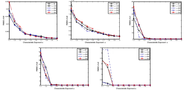
Simulation 2: Characteristic Exponent

In this simulation, the generalized signal to noise ratio is set as GSNR=15 and fractional lower-order moment p₌1.2_{. The influence of characteristic exponent}

α

_{to the performance of these parameters}

is shown in Figure 3. From Figure 3, we can find that the proposed method has better estimation performance when α ≥1.3.

1.1 1.2 1.3 1.4 1.5 1.6 1.7 1.8 1.9 2 0 0.005 0.01 0.015 0.02 0.025

Characteristic Exponent α

R M S E o f b 0

τ =60

τ =120

τ =200

τ =240

τ =300

1.1 1.2 1.3 1.4 1.5 1.6 1.7 1.8 1.9 2 0 0.2 0.4 0.6 0.8 1 1.2 1.4 1.6 1.8x 10

-3

Characteristic Exponent α

R M S E o f a 0

τ =60

τ =120

τ =200

τ =240

τ =300

1.1 1.2 1.3 1.4 1.5 1.6 1.7 1.8 1.9 2 0 10 20 30 40 50 60

Characteristic Exponent α

R M S E o f a 1

τ =60

τ =120

τ =200

τ =240

τ =300

1.1 1.2 1.3 1.4 1.5 1.6 1.7 1.8 1.9 2 0 2 4 6 8 10 12 14 16 18

Characteristic Exponent α

R M S E o f a 2

τ =60

τ =120

τ =200

τ =240

τ =300

1.1 1.2 1.3 1.4 1.5 1.6 1.7 1.8 1.9 2 0 0.5 1 1.5 2 2.5 3 3.5

Characteristic Exponent α

R M S E o f a 3

τ =60

τ =120

τ =200

τ =240

τ =300

Figure 3. Root mean square error versus Characteristic Exponent α.

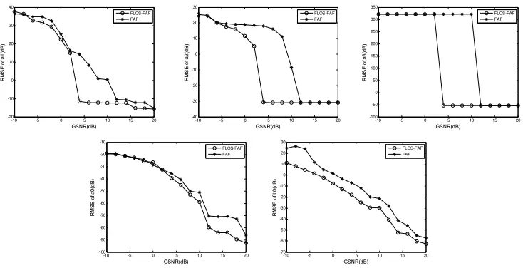
Simulation 3: Compared

In this section, we compare the proposed method and the method of [6]. Based on fractional ambiguity function method is presented in [6]. The method of basing FAF is based second moment. The peak of the fractional ambiguity function of signal is merged by the FAF of noise in the impulsive noise environment, so this method has worse estimation performance. The proposed method use the fractional lower order statistics theory to suppress impulse noise interference. When GSNR≥4, the

-10 -5 0 5 10 15 20 -20

-10 0 10 20 30 40

GSNR(dB) R

M S E o f a 1( dB )

FLOS-FAF FAF

-10 -5 0 5 10 15 20 -40

-30 -20 -10 0 10 20 30

GSNR(dB) R

M S E o f a 2( dB )

FLOS-FAF FAF

-10 -5 0 5 10 15 20 -100

-50 0 50 100 150 200 250 300 350

GSNR(dB) R

M S E o f a 3( dB )

FLOS-FAF FAF

-10 -5 0 5 10 15 20 -100

-90 -80 -70 -60 -50 -40 -30 -20 -10

GSNR(dB) R

M S E o f a 0( dB )

FLOS-FAF FAF

-10 -5 0 5 10 15 20 -70

-60 -50 -40 -30 -20 -10 0 10 20 30

GSNR(dB) R

M S E o f b 0( dB )

[image:6.612.121.488.71.259.2]

FLOS-FAF FAF

Figure 4. Two algorithms comparison.

Conclusion

This paper study parameter estimation method of cubic phase signal. It has been shown that alpha stable processes are better models for impulsive noise than Gaussian processed. Therefore, this paper combined fractional lower order statistics theory and fractional ambiguity function, and proposed FLOS-FAF algorithm. Through searching the peak of FLOS-FAF to estimate parameters of cubic phase signal in impulsive noise. Simulation results demonstrate that the proposed method still has good performance when poor SNR condition exists.

Acknowledgment

This work was partly supported by the National Natural Science Foundation of China under Grants 61401055, the Ph.D Programs Foundation of Liaoning Province of China 20170520421, and the fund of Key Laboratory of marine management technology in State Oceanic Administration People’s Republic of China under Grant 201504. The authors would like to thank the anonymous reviewers for their useful comments and suggestions that significantly improved the paper

References

[1] Y. Li, R. Wu, M. Xing, and Z. Bao, Inverse synthetic aperture radar imaging of ship target with complex motion, IET Radar, Sonar & Navigation. l (2008) 395-403.

[2] S. Barbarossa, V. Petrone, Analysis of polynomial-phase signals by the integrated generalized ambiguity function, IEEE Transactions on Signal Processing. 45(1997) 316-327.

[3] Y.T. Wu, H. So, and H. Liu, Subspace-Based algorithm for parameter estimation of polynomial phase signals, IEEE Transactions on Signal Processing. 56(2008) 4977-4983.

[4] S.Peleg, and B. Friedlander, The Discrete Polynomial Phase Transform, IEEE Transactions on Signal Processing. 43(1995) 1901-1914.

[5] P.O. Shea, A fast algorithm for estimating the parameters of a quadratic FM signal, IEEE Transactions on Signal Processing, 52(2004) 385-393.

[7] S. Pei, J. Ding, Relations between Gabor transforms and fractional Fourier transforms and Their applications for signal processing, IEEE Transactions in Signal Processing. 55(2007) 4839-4850. [8] C.L. Nikias, and M. Shao, Signal processing with alpha stable distributions and applications, New York: John Wiley & Sons Inc,1995, pp. 108-235.

[9] P. Tsakalides and C.L. Nikias, Maximum likelihood localization of sources in noise modeled as a stable process, IEEE Trans. Signal Processing. 43(1995) 2700-2713.

[10] S. Pei, and W. Hsue, The multiple parameter discrete fractional Fourier transform, IEEE Signal Processing Letters. 13(2006) 329-332.