Robust Proportionate Adaptive Filtering Algorithms Against Impulsive Interference

2017 2nd International Conference on Computer, Mechatronics and Electronic Engineering (CMEE 2017) ISBN: 978-1-60595-532-2

Robust Proportionate Adaptive Filtering Algorithms

Against Impulsive Interference

Zhi-hao FU

*

and Yun LIN

Chongqing University of Posts and Telecommunications, Chongqing, 400065, People’s Republic of China

*Correspondence author

Keywords: Sparse adaptive filter, Cost function, Correntropy, Impulsive interference.

Abstract. The Proportionate Normalized Least Mean Square (PNLMS) algorithm, as a popular tool of signal processing, achieves excellent performance for sparse system identification. However, in previous studies, most of the cost functions used in proportionate-type sparse adaptive algorithms are based on the Mean Square Error (MSE) criterion, which is optimal only when the measurement noise is Gaussian. However, when the noise is impulsive noise, the performances of the existing proportionate-type sparse adaptive algorithms deteriorate severely. In this paper, two novel proportionate adaptive algorithms, namely, Proportionate Maximum Correntropy Criterion (PMCC) algorithm based on maximum correntropy criterion algorithm and proportionate normalized least mean square algorithm based on arctangent cost function (P-Arc-NLMS) are proposed to address this problem. The corresponding computational complexity is analyzed. The simulations are done to confirm that the proposed algorithms have advantages, compared with the existing other algorithms proposed against impulsive interference in sparse system identification.

Introduction

The sparse adaptive filter is researched widely in various sparse systems at present, which finds different practical applications, such as network echo cancelation, underwater acoustic communications, wireless multipath channels, and the framework of Compressive Sensing (CS) [1, 3]. A linear system is called sparse if its Finite Impulse Response (FIR) model contains very few active taps that have significantly large magnitude, while other a large number of coefficients are insignificant (i.e. the magnitude equal or close to zero). For example, the network echo channel has an “active” region of only 8–12 ms in a total echo response of about 64–128 ms duration with the “inactive” part accounts for bulk delay due to network loading, encoding and jitter buffer delays [4]. In order to address this problem, some sparse adaptive algorithms such as PNLMS and the Zero-Attracting Least Mean Square (ZALMS), etc., have been proposed in [5, 6], respectively. The variants of PNLMS, PNLMS++, IPNLMS and MPNLMS, are also gradually proposed in [7-9], to improve the convergent rates while ignoring the interferences of impulsive noise, which deteriorates severely the convergent performance of PNLMS algorithm. Although the sparse adaptive algorithms, ZAMCC, Reweighted ZAMCC (RZAMCC) and Correntropy Induced Metric MCC (CIMMCC) algorithms have been presented in [10] to solve this problem to some extent, the convergent rates of these algorithms need be enhanced further to satisfy the different applications.

The PNLMS Algorithm and the Proposed Algorithms

Consider the desired signal d n

( )

that arises from the system identification model d n

( )

=xT

( )

n wo+v n

( )

, where wo is the tap coefficients vector of unknown system,

( )

n

x denotes the input vectorx

( )

n =_x n

( )

, x n

(

−1 ,

)

, x n

(

−L+1

)

_T_{, and}

v n

( )

_{is background}

noise, respectively. The output of filter is

( )

( )

T

( ) ( )

y n =d n −x n w n . The estimated error

is e n

( )

=d n

( )

−xT

( ) ( )

n w n ,

( )

[

0, 2, , 1

]

T L n = w w w ₋

w _{is the estimate of}

o

w at iterationn , respectively. The parameter L is the length of adaptive filter.

The PNLMS Algorithm

The PNLMS algorithm, as a well-known sparse adaptive algorithm proposed in [5], is defined as

(

)

( )

( ) ( ) ( )

( ) ( ) ( )

1 _T n n e n

n n

n n n

+ = +

+

G x

w w

x G x

α

δ (1)

where α is the step-size factor,

δ

>0 is the regularization parameter, andG

( )

n =diag g_{ 0}

( )

n g n₁

( )

g_L−1

( )

n _ is a L L× diagonal matrix, withg n_l

( )

>0,∀n l, . The diagonal elements of G

( )

n as follows:

( )

( )

( )

1 0 l l L i i n g n n − = =

∑

γ

γ (2)

where

γ

_l

( )

n =max_

γ

_min

( )

n , w n_l

( )

_, 0≤ ≤l L−1 . The parameter

γ

_min

( )

n is defined as

γ

_min

( )

n =

ξ

max_

δ

_p, w n₀

( )

,, w_L−1

( )

n _{, and the notation} i _{denotes the absolute value of a} scalar. The parameters ξ and δ_p are positive numbers with typical valuesδ_p =0.01, ξ =5 /L.

The P-Arc-NLMS Algorithm

The cost function of the Arc-NLMS algorithm [11] based on the arctangent function can be expressed as follows:

( )

(

)

( )

( )

2 1 2

arctan( ( ) ) / 2

|| ||

e n

J n E

n α α   =       w

x (3)

where αis the parameter to control the sharpness of the cost function and || ||i 2 denotes 2-norm

of a vector. Therefore, the equation (3) can be improved as follows:

( )

(

)

( )

( )

( )

2 2 2

arctan( ( ) ) / 2

|| ||

e n

J n E n

n α α   =       w G

x (4)

By using the negative stochastic gradient method in equation (4), the weight update formula of proposed algorithm can be written as:

(

)

( )

(

( )

)

( )

( ) ( ) ( )

(

( )

( )

( )

)

2

2 _{2 4} 2

2 2

1

/ /

n n J n

n n n e n n e n n

µ

µ α

+ = − ∇

= + +

w w w

w G x x x

(5)

where µ is the step-size factor.

The PMCC Algorithm

( )

(

)

( )

2

3 exp 2

2

e n

J n E

σ       = −    _{ }  

w (6)

where σ is Gaussian kernel. Similarly, the equation (6) can be changed as follows:

( )

(

)

( )

( )

2

4 exp 2

2

e n

J n E n

σ       = −    _{ }  

w G (7)

By using the positive stochastic gradient method for the equation (7), the weight update formula of the new algorithm can be written as:

(

)

( )

(

( )

)

( )

( ) ( ) ( )

( )

1 4 2 2 1 exp 2

n n J n

e n n n n e n

µ µ σ + = + ∇   = + −   

w w w

w G x (8)

where µ₁ is the step-size factor and 1 2

= µ

µ σ .

Analysis of the Computational Complexity

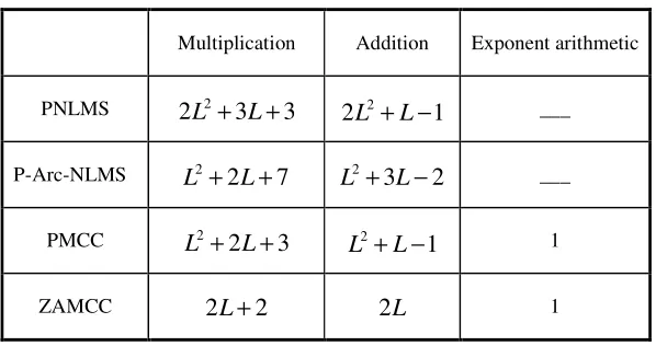
Table.1 summarizes the computational complexity of the PNLMS, P-Arc-NLMS, PMCC, ZAMCC, RZAMCC, and CIMMCC algorithms per iteration. The remarkable point is that the division is seen as multiplication and the subtraction is regarded as addition, and the exponent arithmetic mainly tends to operationexp{ }i _{. Compared with the PNLMS algorithm, the proposed P-Arc-NLMS and}

PMCC algorithms decrease L2+Lmultiplications and L2−2L+1 additions at least, despite of the exponent arithmetic to the PMCC algorithm. Because of introducing the gain-distribution matrixG

( )

n , the proposed P-Arc-NLMS and PMCC algorithms maintain _L2_{multiplications and}

additions in magnitude, which is larger than the computational complexity of the PMCC, ZAMCC, RZAMCC, and CIMMCC algorithms in the case of multiplication and addition. However, for the PMCC, ZAMCC, RZAMCC, and CIMMCC algorithms, the exponent arithmetic is increasing per iteration since exploiting correntropy criterions. Especially, the CIMMCC algorithm contains L+1 exponent arithmetic.

[image:3.612.157.456.567.725.2]

In short, the proposed P-Arc-NLMS has lower computational complexity than that of the PNLMS algorithm. The proposed PMCC slightly increases computational complexity compared with ZAMCC, RZAMCC, and CIMMCC algorithms in the case of multiplication and addition, but contains lower Lexponent arithmetic than that of the CIMMCC algorithm.

Table 1. Summary of the computational complexity.

Multiplication Addition Exponent arithmetic

PNLMS 2L2+3L+3 2

2L +L−1 ___

P-Arc-NLMS _L2_{+2L+7 L}2_{+3L−2 ___}

PMCC 2

2 3

L + L+ _L2_{+L−1 1}

RZAMCC 3L+4 3L 1

CIMMCC 4L+4 2L L+1

Simulation Results

In this section, we make three experiments for three different examples used to identify sparse systems. The 30db Gaussian noise is added to all input signals. And the input signals of the last two examples is disturbed by impulsive noise, which is generated as A k_{i i} [13], where is a Bernoulli

process with a probability of successP k

{

_i=1

}

= p_r, the probability of the occurrence of impulsive noise. The power of A_i is set to

σ

_A2 =1000

σ

_y2 , where

σ

_y2 is the power of the system

outputy=xT

( )

n w_o. The tracking performance is evaluated by the Normalized Mean Square Deviation (NMSD), ₁₀

(

( )

2 2₂

)

2

10 log

= w w

NMSD n / _o . The learning curves are obtained by the

ensemble averages over 100 independent runs.

The Input with Gaussian Noise

In this section, the object is to highlight the advantages of the proposed two algorithms compared with the PNLMS algorithm under Gaussian interference. The reference weight coefficient vectors are defined as follows:

[

]

[

]

1

2

3

0,0,0,1,0,0,0,0,0,0,0,0,0,0,0,1,0,0,0,0,0,0,0,0,0,0,0,0,0,0,0,0

0,0,0,0,0,0,1,0,0,0,0,0,1,0,0,0,0,0,0,0,1,0,0,0,0,0,1,0,0,0,0,0

0,0,0,1,0,0,1,0,0,1,1,0,0,0,1,1,0,0,0,0,0,0,0,0,1,0,0,0,1,0,

T

T

=

= =

=

w

w w

w

o

[

0,0

]

T

    

(9)

The three weight vectors stand for three different channels with the sparsity ratio

(

2 / 32, 4 / 32,8 / 32

)

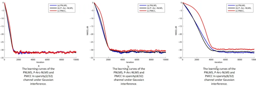
, which are used in the Figure.1.a, Figure.1.b, and Figure.1.c, respectively, to compare the performances of the proposed algorithms and the PNLMS algorithm. Some parameters are set asδ =0.01, ξ =0.5 /L,α=0.01,δ_p =1 /L. In Figure.1.b,a=0.5, and the step-size of the PMCC algorithm is set as 0.02. In Figure.1.a and Figure.1.c, the step-sizes of the PMCC are 0.027, 0.015, respectively. The initial convergent moment is at 1200 iteration in Figure.1.a, 2000 iteration in Figure.1.b, and 4000 iteration in Figure.1.c.

For the condition of the same convergent rate, the P-Arc-NLMS algorithm and the PNLMS algorithm keep the same NMSD while the NMSD of the PMCC algorithm deviates slightly from ones of the PNLMS and the P-Arc-NLMS with the increasing sparsity ratio (from w₁ tow₃).This deviation is reasonable because under MCC the convergence speed may be slow at the initial stage [14] and has little influence in sparse system application.

[image:5.612.86.533.66.217.2]

Figure 1. The learning curves of the PNLMS, P-Arc-NLMS and PMCC in sparsity channel under Gaussian interference.

The Input with Impulsive Noise

[image:5.612.88.520.414.563.2]

When the input is disturbed by the impulsive noise (p_r =0.01), the proposed algorithms, are compared with the ZAMCC, RZAMCC and CIMMCC algorithms. In Figure.2.a, Figure.2.b and Figure.2.c, the parameters are set to ensure that the learning curves have the same convergence rate. Compared with the Figureure Figure.2.a, Figure.2.b and Figure.2.c, the NMSD curves of the PNLMS algorithm deviates severely because of impulsive interference. However, the NMSD curves of the P-Arc-NLMS algorithm and PMCC algorithm stay lower positions, which are lower than those of the ZAMCC, RZAMCC and CIMMCC algorithms. From Figure.2.b to Figure.2.c, with the increasing sparsity ratio of the system, the ZAMCC and RZAMCC algorithms are gradually close to proposed algorithms in the case of learning curves. Simultaneously, for the NMSD curves, the CIMMCC algorithm mostly stays the same position with the proposed algorithms except that the NMSD curve of the CIMMCC algorithm deviates up in Figure.2.b.

Figure 2. The learning curves of the PNLMS, P-Arc-NLMS, PMCC, ZAMCC, RZAMCC and CIMMCC in sparsity channel under impulsive interference.

From the simulation results, the PMCC algorithm and the P-Arc-NLMS algorithm in a non-Gaussian impulsive noise environment can also outperform the ZAMCC algorithm and the RZAMCC algorithm in the case of convergence rate. Simultaneously, the proposed algorithms at least ensure that the performance stays consistent with that of the CIMMCC algorithm in different sparsity ratio systems.

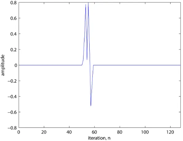
The Proposed Algorithms Used in Random Sparse Echo Channel

[image:6.612.144.442.134.364.2]

PNLMS algorithm is highest 10dB than those of the proposed algorithms because the PNLMS algorithm is not robust under impulsive noise environment; The ZAMCC, RZAMCC, and CIMMCC algorithms are highest 2dB at least than the proposed algorithms in case of the learning curves, which demonstrates that the proposed algorithms have great convergent performances against impulsive interference to identify sparse echo channel.

[image:6.612.161.457.387.617.2]

Figure 3. Impulse response of artificially generated sparse echo channels.

Figure 4. The learning curves of the PNLMS, P-Arc-NLMS, PMCC, ZAMCC, RZAMCC and CIMMCC with the weight of the Figure.3 under impulsive interference.

Conclusion

complexity compared with existing sparse adaptive algorithms. Simultaneously, the simulation results also show that the proposed algorithm achieves a better performance, the better ability of immunity to impulsive interference, in terms of the tracking stable NMSD values, compared with the ZAMCC, RZAMCC and CIMMCC algorithm. Therefore, it is more potential to promote the proportionate-type algorithm applied to different sparse adaptive system identifications.

Reference

[1] Huang Y, Benesty J and Chen J. “Acoustic MIMO signal processing,” Springer Science & Business Media, 2006.

[2] Paleologu C, Benesty J, and Ciochina S. “Sparse adaptive filters for echo cancellation.” Synthesis Lectures on Speech and Audio Processing 6.1 (2010): 1-124.

[3] Jin J, Gu Y, and Mei S. “A stochastic gradient approach on compressive sensing signal reconstruction based on adaptive filtering framework.” Selected Topics in Signal Processing, IEEE Journal of 4.2 (2010): 409-420.

[4] Das R L and Chakraborty M. “Sparse adaptive filters - An overview and some new results,” 2012 IEEE International Symposium on Circuits and Systems (ISCAS), pp. 2745-2748, Seoul, 2012.

[5] Duttweiler, Donald L. “Proportionate normalized least-mean-squares adaptation in echo cancelers.” Speech and Audio Processing, IEEE Transactions on 8.5 (2000): 508-518.

[6] Yilun C, Gu Y, and Hero III A O. “Sparse LMS for system identification.” Acoustics, Speech and Signal Processing, 2009. ICASSP 2009. IEEE International Conference on. IEEE, 2009.

[7] Gay S L. “An efficient, fast converging adaptive filter for network echo cancellation.” Signals, Systems & Computers, 1998. Conference Record of the Thirty-Second Asilomar Conference on. Vol. 1. IEEE, 1998.

[8] Benesty J and Gay S L. “An improved PNLMS algorithm.”Acoustics, Speech, and Signal Processing (ICASSP), 2002 IEEE International Conference on. Vol. 2. IEEE, 2002.

[9] Deng H and Doroslovacki M. “Improving convergence of the PNLMS algorithm for sparse impulse response identification.” Signal Processing Letters, IEEE 12.3 (2005): 181-184.

[10] Ma W, et al. “Maximum correntropy criterion based sparse adaptive filtering algorithms for robust channel estimation under non-Gaussian environments.” Journal of the Franklin Institute (2015).

[11] Zeng J, Yun L, and Liming S. “A Normalized Least Mean Square Algorithm Based on the Arctangent Cost Function Robust Against Impulsive Interference.” Circuits, Systems, and Signal Processing (2015): 1-8.

[12] Singh A and Principe J C. “Using correntropy as a cost function in linear adaptive filters.” Neural Networks, 2009. IJCNN 2009. International Joint Conference on. IEEE, 2009.

[13] Shi L and Yun L. “Convex Combination of Adaptive Filters under the Maximum Correntropy Criterion in Impulsive Interference.” Signal Processing Letters, IEEE 21.11 (2014): 1385-1388.