2017 International Conference on Computer Science and Application Engineering (CSAE 2017) ISBN: 978-1-60595-505-6
Internet Traffic Forecasting using Boosting LSTM Method
Guangkuo Bian*, Jun Liu and Wenhui Lin
School of Information and Communication Engineering, Beijing University of Posts & Telecommunications Address: No.10 Xitucheng Rd, Haidian District,
100876 Beijing, China
ABSTRACT
As Internet traffic is a kind of time series, the algorithms which are suitable for time series forecasting are also appropriate for Internet traffic. We study approaches for time series prediction firstly and then apply the algorithms to Internet traffic prediction in this paper. We present an ensemble method based on Long Short-Term Memory (LSTM) Network method for time series prediction with the aim of increasing the prediction accuracy of Internet traffic. We use AdaBoost algorithm to boost LSTM method because AdaBoost algorithm is the most widely used boosting algorithm. However, original AdaBoost algorithm is not suitable for prediction, in view of this fact, we use modified AdaBoost algorithm to be combined with LSTM in this paper. We use two data sets to experiment, and the results show that AdaBoost-LSTM algorithm is more accurate than single LSTM algorithm and even better than ARIMA in some situations. At last, we apply AdaBoost-LSTM algorithm to forecast the Internet traffic.
INTRODUCTION
Time series prediction can solve many problems in different domains ranging from finance, dynamic systems control and marketing. Moreover, the reliable prediction of future values of Internet traffic as a type of time series plays an important role in network security and resource management.
As Internet traffic is a kind of time series, time series prediction methods are always suitable for Internet traffic forecasting. In this way, we do researches on general time series prediction firstly and apply the algorithms to predict Internet traffic next.
In time series prediction domain, there have been many forecasting methods. They can be classified into two kinds: linear and nonlinear prediction algorithms. Linear forecasting algorithms include ARMA/ARIMA model 123 and Holt-Winters methods while nonlinear forecasting algorithms contain neural networks 45. It indicates that nonlinear forecasting algorithms using neural networks perform better than linear prediction algorithms such as ARIMA in 6. All these prediction methods can be applied to Internet traffic flow.
the modified AdaBoost algorithm ensemble with LSTM network called “AdaBoost-LSTM” for time series forecasting problems to improve the performance of single LSTM algorithm and apply this algorithm to Internet traffic prediction in this paper. To verify the accuracy of the method, two time series problems are employed in the experiment.
Conventional RNN has the exploding gradient and vanishing problems. LSTM, one special network of RNN, has been proposed to improve the performance of RNN and address the problems of conventional RNN. In some situations, an LSTM can offer a more accurate result in predicting non-linear time series.
There are many boosting algorithms, the most widely used algorithm is AdaBoost algorithm. AdaBoost algorithm trains different weak classifiers based on the same training set and combine these classifiers into a single strong classifier, the ensemble model has a good performance on all samples. However, since original AdaBoost algorithm is only suitable for classification but not regression, we modify original AdaBoost algorithm to make it appropriate for time series prediction.
In this paper, the concept of LSTM networks as well as RNN networks will be described in section 2. In section 3, we will introduce AdaBoost algorithm and in section 4, the modification of AdaBoost algorithm will be proposed. In section 5, AdaBoost-LSTM algorithm will be described. We use AdaBoost-LSTM algorithm to forecast future values on two benchmark data sets and then analyze the results and compare the results with those using ARIMA model in section 6. Then the method we proposed will be applied to Internet traffic time series prediction in section 7. And finally, a conclusion is included at last.
NEURAL NETWORKS Recurrent Neural Networks
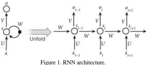
[image:2.612.176.418.550.658.2]Since Long Short-Term Memory Networks (LSTMs) are a special kind of Recurrent Neural Networks (RNNs), we introduce RNNs firstly. RNNs are called recurrent because the connections between units compose a cycle. The previous computations can also affect the output being. The figure below shows the architecture of a typical RNN:
Figure 1. RNN architecture.
𝑠𝑡= 𝑓(𝑈𝑥𝑡+ 𝑊𝑠𝑡−1) where the function f is a nonlinear function such as tanh. 𝑜𝑡 is computed as 𝑜𝑡 = 𝑠𝑜𝑓𝑡𝑚𝑎𝑥(𝑉𝑠𝑡).
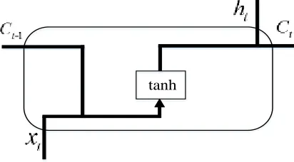
All recurrent neural networks are composed of a chain of repeating modules of neural network. In order to explain LSTMs intuitively, we provide a Figure 2 which shows the repeating module of standard RNNs below 12. It shows that the repeating module has a very simple structure.
[image:3.612.194.400.157.271.2]tanh
Figure 2. The repeating module of RNNs.
Long Short-Term Memory Networks
Above is a brief introduction of RNNs, the concept of LSTMs is described next. Long Short-Term Memory (LSTM) was proposed by Sepp Hochreiter and Jürgen Schmidhuber [13] and improved by Felix Gers et al in 2000 [14]. It works especially well in a variety of domains such as classification problems and even time series prediction problems.
Standard Recurrent Neural Networks (RNNs) suffer from vanishing and exploding gradient point problems. LSTMs are designed to address these problems. LSTMs deal with these problems by introducing new gates, such as input and forget gates, which allow for a better control over the gradient flow and enable better preservation of long-range dependencies.
[image:3.612.194.402.550.667.2]Same as RNNs, LSTMs also have a repeating module. But the repeating module is different from RNNs. The architecture of the repeating module is complicated.There are four neural network layers in LSTMs including input layer, gate layer, cell layer and output layer rather than single simple tanh layer. The repeating module is shown in Figure 3 as below [12].
× +
σ σ
×
tanh σ × tanh
For a given input sequence 𝑥 = (𝑥1, 𝑥2, … , 𝑥𝑇), an LSTM network computes an output sequence ℎ = (ℎ1, ℎ2, … , ℎ𝑇). When we take the last output ℎ𝑡−1, the last cell state 𝐶𝑡−1 and the current input 𝑥𝑡 as inputs, we can use the following equations to obtain the current output ℎ𝑡 and the current cell state 𝐶𝑡, then ℎ𝑡 and 𝐶𝑡 will be used in the next iteration. The output sequence ℎ = (ℎ1, ℎ2, … , ℎ𝑇) is calculated iteratively from t = 1 to T with the following equations.
𝑖𝑡 = σ(𝑊𝑖 ∙ [ℎ𝑡−1, 𝑥𝑡] + 𝑏𝑖) (1)
𝑓𝑡 = σ(𝑊𝑓∙ [ℎ𝑡−1, 𝑥𝑡] + 𝑏𝑓) (2)
𝐶̃𝑡= 𝑡𝑎𝑛ℎ (𝑊𝑐∙ [ℎ𝑡−1, 𝑥𝑡] + 𝑏𝑐) (3)
𝐶𝑡 = 𝑓𝑡∗ 𝐶𝑡−1+ 𝑖𝑡∗ 𝐶̃𝑡 (4)
𝑜𝑡 = σ(𝑊𝑜[ℎ𝑡−1, 𝑥𝑡] + 𝑏𝑜) (5)
ℎ𝑡= 𝑜𝑡∗ 𝑡𝑎𝑛ℎ (𝐶𝑡) (6)
Here the W terms signify weight matrices, for example, 𝑊𝑖 denotes the matrix of
weights from the input gate to the input, is sigmoid function, and the b terms represent bias vectors. i is the input gate while f is the forget gate, o is the output gate, C
represent the cell state and ℎ𝑡 is the output.
ADABOOST
There are many boosting algorithms, the most widely used algorithm is AdaBoost. AdaBoost is a method that combines many simple weak learners into a strong classifier. The final output is calculated as combining the output of weak learners into weight sum. Many other types of learning algorithms can be combined into one model using AdaBoost algorithm to improve their performance. The final model is a strong model when every weak learner satisfies that the performance of it is better than random guessing. The detail of AdaBoost algorithm will be introduced next.
Here we are given a training set, (𝑥𝑖, 𝑦𝑖), 𝑖 = 1, … , 𝑛 as inputs where 𝑥𝑖 is a sample
in domain X, 𝑋 = {𝑥𝑖, 𝑖 = 1, … , 𝑛}, and 𝑦𝑖 ∈ {−1, +1} is a label associate with 𝑥𝑖.
AdaBoost trains for K iterations to get K weak learners to combine. At each iteration
k=1, ..., K, a set of weights on the training set is assigned by the algorithm. For k=1, all the weights are set equally. 𝐷𝑘(𝑖) represents the weight of training sample i at iteration
k. Then the weak learner trains itself with this 𝐷𝑘. At next iteration, the learner will pay
more attention to the hard samples in the training set by increasing the weight of incorrectly classified samples and decreasing the weight of correctly classified samples. At the iteration, the weak learner has to compute a weak hypothesis ℎ𝑘: X → {−1, +1}
with low weighted error ε𝑘 relative to 𝐷𝑘.The final hypothesis H is a linear combination of the weak hypothesis ℎ𝑘 , calculated as a weighted sum of
Given: Initialize:
Iterate: For k=1,...,K:
1. Train weak learner using distribution
2. Get hypothesis, , with the error function , with respect to
3. Choose
4. Reweight
Where is a normalization factor.
Output: The final hypothesis
k D k
h
k] ) ( [
Pri~D k i i
k k h x y
) 1 ln( 2 1 k k k a ) ( 1 i Dk k i k i k k k Z x h y a i D iD 1() ()exp( ( ))
k Z
n i i k i k kk D i a yh x
Z 1 )) ( exp( ) (
K k k kh xa sign x H 1 )) ( ( ( ) ( ) ,
(xi yi xiX,X {xi,i1,...,n},yi{1,1}
k
D n
[image:5.612.122.484.46.662.2]i D1()1/
Figure 4. The AdaBoost method.
Given: Initialize:
Iterate: For k=1,...,K:
1. Train weak learner using distribution
2. Get hypothesis, , with the error function , in regard to .Error function can be the difference between the actual and predicted values or other error functions which is then weighted by
3. Choose
4. Reweight
Where is a normalization factor.
Output: The final hypothesis
n i D1()1/
k D k Z k D k
h
k
k D k
) 1 ln( 2 1 k k k a
) ( 1 iDk
k k k k k k
Z
i
a
i
D
i
D
1(
)
(
)
exp(
(
)
/
)
n i k k k kk
D
i
a
i
Z
1)
/
)
(
exp(
)
(
K k K k k kkh x a
a x H 1 1 / )) ( ( ) ( ) ,
[image:5.612.125.483.55.358.2](xi yi xiX,X {xi,i1,...,n};yiY,Y {yi,i1,...,n}
MODIFIED ADABOOST
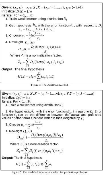
Since we are studying on time series prediction problems, here we are interested in how to use AdaBoost algorithm for prediction. It is generally harder to solve prediction problems using boosting methods than solving classification problems. The outputs of classifiers are classes while the outputs of predictors are real value rather than classes. Original AdaBoost algorithm is not suitable for prediction problems. To suit time series forecasting problems, modified AdaBoost algorithm were proposed in 101115.The modified AdaBoost algorithm we use for prediction in this paper is shown in Figure 5.
There are several differences between modified AdaBoost algorithm and original AdaBoost algorithm. Modified AdaBoost algorithm takes a training set, (𝑥𝑖, 𝑦𝑖), 𝑖 = 1, … , 𝑛 as inputs where 𝑥𝑖 is an instance in domain X, 𝑋 = {𝑥𝑖, 𝑖 = 1, … , 𝑛}, and 𝑦𝑖 is an instance in domain Y associated with 𝑥𝑖, 𝑌 = {𝑦𝑖, 𝑖 = 1, … , 𝑛}. Different from original AdaBoost algorithm, 𝑦𝑖in modified AdaBoost is real-valued. At iteration k, the LSTM network is trained using 𝐷𝑘(𝑖) over the training set. At first, 𝐷1(𝑖) are set equally, 𝐷1(𝑖) = 1/𝑛. Then the network computes the weak hypothesis ℎ𝑘 using error
function 𝜀𝑘, in regard to 𝐷𝑘. 𝜀𝑘 is a user-defined unit error function weighted by 𝐷𝑘 in
modified AdaBoost algorithm, for instance, 𝜀𝑘= (𝑦 − 𝑦𝑝𝑟𝑒𝑑)2, while 𝜀
𝑘 is the
summation of the probabilities of incorrectly classified samples in original AdaBoost algorithm. 𝐷𝑘+1 is reweighted by changing the weight of samples in accordance with the error function next. A normalization factor 𝑍𝑘 is used to constrain 𝐷𝑘+1 as a distribution, Since 𝐷𝑘+1 is reweighted at each iteration, network is forced to focus on the harder samples. At last, the final output is computed by taking the outputs of trained networks and combining them together according to their parameter 𝑎𝑘 which reflects the importance of the network.
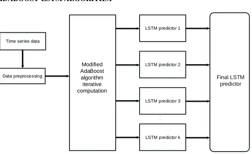
ADABOOST-LSTM ALGORITHM
LSTM predictor 1
LSTM predictor 2
LSTM predictor 3
LSTM predictor k Data preprocessing
Time series data
Modified AdaBoost algorithm iterative computation
. . .
[image:6.612.99.500.441.687.2]Final LSTM predictor
The AdaBoost-LSTM algorithm which we proposed in this paper is shown in Figure 6, we use the modified AdaBoost method to iteratively train LSTM networks, after k iterations, we get k weak LSTM predictors, then we combine these k predictors into one predictor to forecast the Internet traffic data. In section 6, We have done some experiments using AdaBoost-LSTM algorithm.
EXPERIMENTAL RESULTS
In this paper, two data sets are used to verify the effectiveness of AdaBoost-LSTM algorithm. One is a sunspot data set and another is a random data set. All the associated programs are written in Python, the version of Python is 3.7.
We use the root mean squared error (RMSE) to judge the performance of each algorithm and compare with each other. RMSE is computed as follows[16]:
RMSE = √1
𝑛∑ |𝑦𝑡− 𝑦𝑝𝑟𝑒| 2 𝑛
𝑡=1 (7)
Here n represents the size of the test set, 𝑦𝑡 and 𝑦𝑝𝑟𝑒 respectively represent the actual value and the forecasted value.
For each data set, we firstly display the origin data using diagram and then compare our obtained results with other methods using tabular form. At last we use some graphs to show the test and forecasted values. In every forecast graph, the actual observations are represented by the solid line while the forecasted observations are plotted using the dotted line.
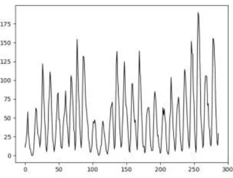
[image:7.612.181.409.463.638.2]The Wolf’s Sunspot Dataset
Figure 7. Wolf’s sunspot data series (1700-1987).
and the remaining 67 (i.e., 1921 to 1987) are used for the test data set. In [16], it has been verified that AR (9) is the optimal ARIMA model for this series. We have fitted to the sunspots series using AR(9), LSTM (60 hidden units, 200 epochs), AdaBoost-LSTM (15 boost rounds, 60 hidden units, 200 epochs) and SVM. We measure the performance with RMSE, the results are shown in the TABLE I:
TABLE I. SUNSPOT SERIES PREDICTION RESULTS.
Method RMSE
AR(9) 21.99
LSTM 25.44
AdaBoost-LSTM 22.35 SVM
(
𝐶 = 43.6432 𝜎 = 290.1945 𝑛 = 9, 𝑁 = 212
) 28.16
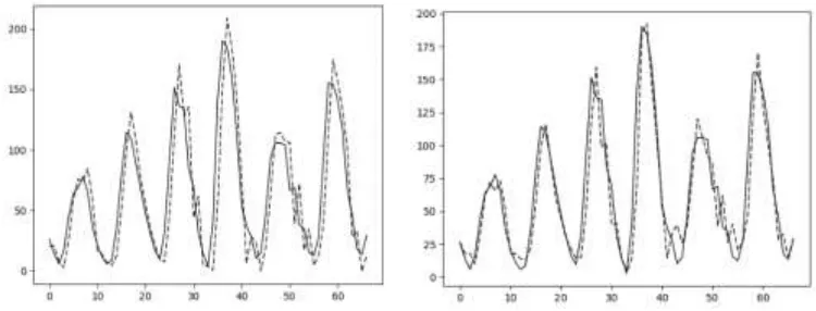
It is easy to see that the forecasting performance of AR(9) is the best in this test for the sunspot series from the above table. AdaBoost-LSTM is better than LSTM and they are all better than SVM algorithm. Here we just show LSTM and AdaBoost-LSTM forecast diagrams, other models’ forecast diagrams can be found in 16. The two prediction diagrams for the sunspot series are shown in the figures below:
[image:8.612.105.480.368.511.2]Figure 8. Prediction of Wolf’s sunspot using LSTM algorithm.
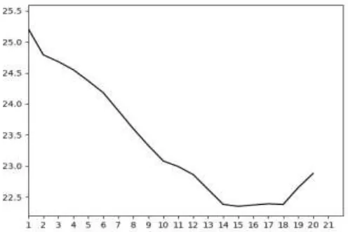
Figure 10. RMSE of AdaBoost-LSTM algorithm with different values of AdaBoost round.
There are 60 hidden units in the LSTM cell, and we specify 200 epochs to train the model. From Figure 8 and Figure 9, we can see that predicting test set with AdaBoost-LSTM algorithm is better than single LSTM algorithm with performance improvement around 12.15%. In Figure 10, AdaBoost-LSTM algorithm is satisfying if the AdaBoost round is small but is upset if the training round is big. Here we can see that the performance becomes worse if AdaBoost round is bigger than 15. The reason of this phenomenon is that the model is overfitting as the AdaBoost round is big.
[image:9.612.168.416.74.240.2]The Random Dataset
Figure 11. Random data set.
AdaBoost-LSTM algorithm. Here, we use 3 rounds to boost and use 200 epochs to train. There are 60 hidden units in the LSTM cell. Naive forecast is a good baseline forecast where the observation from the prior time step t-1 is used to predict the observation at the current time step t. The performance of two algorithms are shown as below TABLE II:
TABLE II. FORECAST RESULTS FOR RANDOM SERIES.
Method RMSE
Naive 4.85
LSTM 4.75
AdaBoost-LSTM 4.50
From the above table, we can see that AdaBoost-LSTM and LSTM algorithm are both better than Naive model and AdaBoost-LSTM algorithm is greater than LSTM with performance improvement around 7.21%.
APPLY ADABOOST-LSTM ALGORITHM TO INTERNET TRAFFIC PREDICTION
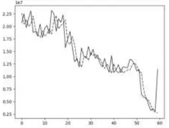
After above works, we have proved that AdaBoost-LSTM algorithm is better than the standard LSTM algorithm. In purpose of forecasting the Internet traffic time series, we apply AdaBoost-LSTM algorithm to the Internet traffic and forecast its future values. The Internet traffic data series we have is shown in Figure 12.
The data series is periodic and nonlinear, it represents the Internet traffic in our lab from August 1st, 2015 to August 5th, 2015. We use the Internet traffic of the last hour in last day as the test dataset and the remaining as the training dataset. Figure 13 illustrates the prediction result.
CONCLUSIONS
After experimenting and analyzing, there are some conclusions we can obtain as follows:
[image:10.612.311.484.334.465.2] AdaBoost-LSTM is proved to be better than the standard LSTM algorithm, marked by the performance increase on all of the testing scenarios.
[image:10.612.106.281.336.469.2] AdaBoost-LSTM is easy to configure, there are just few hyperparameters needed to fit, such as AdaBoost round, the number of hidden units in the LSTM cell and training epochs, on the contrast, ARIMA algorithm needs to know which model should be used before training with ACF and PACF analyzing.
ACKNOWLEDGEMENT
This work is supported in part by Fundamental Research Funds for the Central University under Grant No.2016RCGD09 and 111 Project of China (B08004, B17007). This work is conducted on the platform of Center for Data Science of Beijing
University of Posts and Telecommunications.
REFERENCES
1. P. Cortez, M. Rio, M. Rocha, and P. Sousa. 2006. “Internet Traffic Forecasting using Neural Networks,” International Joint Conference on Neural Networks, pp. 2635-2642.
2. H. Feng, and Y. Shu. 2005. “Study on Network Traffic Prediction Techniques,” International Conference on Wireless Communications, pp. 1041-1044.
3. J. Dai, and J. Li. 2009. “VBR MPEG Video Traffic Dynamic Prediction Based on the Modeling and Forecast of Time Series”, pp. 1752-1757.
4. V. B. Dharmadhikari, and J. D. Gavade. 2010. “An NN Approach for MPEG Video Traffic Prediction,” 2nd International Conference on Software Technology and Engineering, pp. V1-57V1-61.
5. A. Abdennour. 2006. “Evaluation of neural network architectures for MPEG-4 video traffic prediction,” IEEE Transactions on Broadcasting, pp. 184-192.
6. Barabas, and Melinda, et al. 2011. “Evaluation of network traffic prediction based on neural networks with multi-task learning and multiresolution decomposition,” Intelligent Computer Communication and Processing (ICCP), 2011 IEEE International Conference on, pp. 95-102. 7. P.G. Madhavan. 2002. “Recurrent neural network for time series prediction,” Engineering in
Medicine and Biology Society, pp. 250-255.
8. Y.X. Tian, and P. Li. 2016. “Predicting Short-Term Traffic Flow by Long Short-Term Memory Recurrent Neural Network,” Smart City/SocialCom/SustainCom (SmartCity), pp. 153-158. 9. Z. Zhao, W.H. Chen, and X.M. Wu. 2017. “LSTM network: a deep learning approach for
short-term traffic forecast,” pp. 68-75.
10. R. Bone, M. Assaad, and H. Cardot. 2008. “A New Boosting Algorithm for Improved time-series forecasting with Recurrent Neural Networks,” Information Fusion, 9, pp. 41-55.
11. R. Soelaiman, A. Martoyo, and Y. Purwananto. 2009. “Implementation of recurrent neural network and boosting method for time-series forecasting,” ICICI-BME, pp. 1-8.
12. Olah, C. 2015. Understanding LSTM Networks. [online] Available at: http://colah.github.io/posts/2015-08-Understanding-LSTMs/ [Accessed 5 July 2017].
13. S. Hochreiter, and J. Schmidhuber. 1997. “Long Short-Term Memory,” Neural Computation, pp. 1735-1780.
14. F.A. Gers, J. Schmidhuber and F. Cummins. 2000. “Learning to Forget: Continual Prediction with LSTM,” Neural Computation, pp. 2451-2471.
15. C.P. Lim and W.Y. Goh. 2006. “The Application of an Ensemble of Boosted Elman Networks to Time Series Prediction: A Benchmark Study,” International Journal of Computational Intelligence, 3(2), pp. 119-126.
16. R. Adhikari, and R.K. Agrawal. “An Introductory Study on Time Series Modeling and Forecasting,” arXiv: 1302. 6613v1.