BIROn - Birkbeck Institutional Research Online
Garratt, Anthony and Mitchell, J. and Vahey, S.P. (2009) Measuring output
gap uncertainty. Working Paper. Birkbeck College, University of London,
London, UK.
Downloaded from:
Usage Guidelines:
Please refer to usage guidelines at or alternatively
ISSN 1745-8587
Birkbeck Workin
g
Pa
p
ers in Economics & Finance
School of Economics, Mathematics and Statistics
BWPEF 0909
Measuring Output Gap Uncertainty
Anthony Garratt
Birkbeck, University of London
James Mitchell
NIESR
Shaun P. Vahey
Melbourne Business School
Measuring Output Gap Uncertainty
∗
Anthony Garratt
(Birkbeck College)
James Mitchell
(NIESR)
Shaun P. Vahey
(Melbourne Business School)
October 19, 2009
Abstract
We propose a methodology for producing density forecasts for the output gap in real time using a large number of vector autoregessions in inflation and output gap measures. Density combination utilizes a linear mixture of experts framework to produce potentially non-Gaussian ensemble densities for the unobserved output gap. In our application, we show that data revisions alter substantially our proba-bilistic assessments of the output gap using a variety of output gap measures derived from univariate detrendingfilters. The resulting ensemble produces well-calibrated forecast densities for US inflation in real time, in contrast to those from simple uni-variate autoregressions which ignore the contribution of the output gap. Combining evidence from both linear trends and more flexible univariate detrending filters in-duces strong multi-modality in the predictive densities for the unobserved output gap. The peaks associated with these two detrending methodologies indicate output gaps of opposite sign for some observations, reflecting the pervasive nature of model uncertainty in our US data.
Keywords: Output gap uncertainty; Density combination; Ensemble Forecasting; VAR models
JEL codes: C32; C53; E37
1
Introduction
The formulation of monetary policy in many central banks gives prominence to the output gap despite its uncertainty as documented by Orphanides and van Norden (2002, 2005). Their work establishes both the unreliability in real time of output gap (point) measure-ments implied by a variety of well-known filters, and the associated difficulties of using those imprecise measurements to forecast inflation in real time.
This paper provides a methodology that allows the researcher to gauge the uncertainty in output gap measurements across a number of detrending methods. Given the difficulties of estimating stable empirical relationships in short samples, and the presence of macro data revisions, estimates of the output gap based on a single detrending method are fragile; see, for example, Watson (2007). Whereas Orphanides and van Norden (2002) focus on the sensitivities of particular output gap measures, we focus on the uncertainty across different measures and model specifications.
Our ensemble methodology constructs real-time predictive densities for the unobserved output gap using many component bivariate vector autoregressive (VAR) models. Com-ponent models are differentiated by the detrending measure used to derive the output gap, and auxiliary assumptions (such as lag lengths and break dates). We combine fore-cast densities from component models using a linear mixture of experts (also known as the linear opinion pool); see Timmermann (2006) for a discussion of density combination methods. For each component VAR in inflation and a single output gap measure, we mea-sure the Kullback-Leibler “distance” between the real-time h-step ahead inflation forecast density and the true but unknown density using the logarithmic score. Our linear opinion pool builds potentially non-Gaussian forecast densities for inflation and the unobserved output gap from the many components using Kullback-Leibler distance weights for
in-flation. In this way, our output gap predictive densities (predictives) reflect the ability of the ensemble to predict inflation; following the idea in Laubach and Williams (2003), we use the Phillips curve to inform our analysis of real-time output gaps. The ensemble densities for the unobserved output gap reveal the real-time uncertainty about the output gap (h-steps ahead) by construction. In so doing, we focus on predictive density combi-nation over the entire model space, rather than on the difficulties of using, or selecting, a particular detrending method.
real-time data. For example, policymakers using real-time data in the late 1990s would have concluded that the probability of above trend output (a boom) was much smaller than subsequently indicated once the data were revised. We also show that a simple autoregressive benchmark (i.e., a forecasting model without the output gap) produces poorly calibrated densities for US inflation, despite its competitive performance in terms of point forecast accuracy. Put differently, output gaps matter for forecasting inflation densities. Broadening the scope of our applied work to consider linear time trends in output, as well as moreflexible trends, produces a very different assessment of the latent output gap variable using a “grand ensemble” which combines the two trend types. For our US data, this indicates strong multi-modality for the output gap. Our example draws attention to the risk attached to business cycle assessments based on the “best” single (univariate) detrending method.
The remainder of this paper is structured as follows. In Section 2 we describe our methods for forecast density combination used to gauge the uncertainty in the latent output gap. In Section 3, we apply our methodology to US data to produce output gap densities. In the final Section, we conclude and discuss the scope for future research in this area.
2
Methodology
In this Section of the paper, we describe our methodology for gauging the model un-certainty in the output gap. We begin by defining a well-known model space for the component bivariate VARs, broadening slightly the space of van Norden and Orphanides (2005) to allow scope for a single structural break of unknown timing in the inflation equa-tion. Then we describe how to construct the ensemble predictives from the component densities.
2.1
Component Model Space
Following van Norden and Orphanides (2005), we consider linear Phillips curve forecasting models of the form:
πt+h =αj1+ P
X
p=0
βj1,pπt−p + P
X
p=0 γj1,py
j t−p+ε
j
1,t+h, (1)
where inflation is denoted πt and the various output gap measures are denoted yjt, with
j = 1, . . . , J; P + 1denotes the maximum number of lags in inflation and the output gap
measures, andh is the forecast horizon.
We augment this specification with the corresponding output gap equation:
ytj+h =αj2+
P
X
p=0
βj2,pπt−p + P
X
p=0
to create a bivariate VAR system. For simplicity, we assume that the lag structure is identical in the two equation VAR system.
We emphasize that although each VAR component uses a particular output gap mea-sure, our aim is not tofind the “best” single measure of the output gap. Rather, we wish to build ensemble forecast densities for the unobserved output gap variable, conditional on a number of candidate measures. In doing so, we interpret the various output gap measurements as deviating from the “true” but unobserved output gap by more than white noise measurement error.
The two-equation recursive structure described by equations (1) and (2) is common to many more detailed models of inflation determination. For example, Rudebusch and Svensson (2002) and Laubach and Williams (2003) start with similar bivariate struc-tures, and add additional explanatory relationships and restrictions; Garratt et al (2009) consider bigger VARs to assess whether money causes inflation and output. In princi-ple, additional equations and the imposition of identifying conditions pose no conceptual problems for our methodology, although the computational burden would increase. We prefer to restrict our attention to a two-equation model space which, as Sims (2008) notes, lies at the heart of many explanations of inflation determination.
A number of papers, including Stock and Watson (1999), have argued that the rela-tionships between inflation and output gaps altered during the shift from (what is often referred to as) the US Great Inflation to the Great Moderation. Hence, for output gap measurement applications on contemporary samples, the model space must accommodate structural breaks of unknown timing in a computationally convenient manner. We take a pragmatic response and consider every feasible single break date, assuming a single coincident break in the conditional mean and variance for both equations. This raises the potential number of models dramatically since, in effect, each candidate break date defines a new component VAR. We also note that there is uncertainty over the number of lags to include in the system. If we haveJ output gap measures, and for any givenyjt, we haveK different variants defined over different values of the maximum lag length and the location of the break date, then in total we have N =J ×K models, and N associated forecasts of inflation and the output gap.
2.2
Ensemble Construction
Monetary policymakers often focus on the forecast performance for inflation when con-sidering output gap measures in practice. In our ensemble approach, we construct the output gap predictives based on the forecast densities for inflation of our many compo-nent VAR models.1 We combine the many component forecast densities using the linear mixture of experts, also known as the linear opinion pool; see Timmermann (2006). Each bivariate component VAR is scored for the Kullback-Leibler distance between the real-time h-step ahead inflation forecast density and the true but unknown density. Density combination, via the linear opinion pool, then constructs the ensemble forecast densities
for inflation and the unobserved output gap using Kullback-Leibler distance weights for inflation, based on the logarithmic scores of the forecast densities. The resulting out-put gap densities reflect the model uncertainty in the many component specifications, including the uncertainty regarding the measure of the output gap.
More formally, we consider a monetary policy maker seeking to aggregate forecasts supplied by “experts”’, each of which uses a unique bivariate VAR specification to produce a forecast density for inflation. Given i = 1, . . . , N VAR specifications, the combined densities are defined by the convex combination:2
p(πτ ,h) =
N
X
i=1
wi,τ ,h g(πτ ,h |Ii,τ), τ =τ , . . . , τ , (3)
where g(πτ ,h | Ii,τ) are the h-step ahead forecast densities from model i, i = 1, . . . , N of inflation πτ, conditional on the information set Iτ (the same form of equation is also used when constructing output gap combined densities). The publication delay in the production of real-time data ensures that this information set contains lagged variables, here assumed to be datedτ−1and earlier. For simplicity, we assume that each individual model is used to produce h-step ahead forecasts via the direct approach; see the discussion by Marcellino, Stock and Watson (2003). Hence, the macro variables used to produce an h-step ahead forecast density forτ are dated τ−h. In the case whereh= 1, the forecast effectively becomes a “nowcast”. The non-negative weights,wi,τ ,h, in this finite mixture sum to unity.3 Furthermore, the weights may change with each recursion in the evaluation period τ =τ , . . . , τ .
Each component VAR considered can be estimated by maximum likelihood for the Gaussian linear model to provide each component forecast density g(·). However, the ensemble density defined by equation (3) will be a mixture of the component densi-ties. Therefore, the linear opinion pool accommodates potentially severe departures from Gaussian behaviour. For example, multi-modal forecast densities for the output gap are feasible. This feature allows us to explore the extent to which various measurements of the output gap shape the ensemble forecast densities. Kascha and Ravazzolo (2009) dis-cuss logarithmic opinion pooling which forces the forecast densities to be unimodal, and masks the tension between forecasts from various component models.
We propose the weights be based on the fit of the individual component forecast densities. Following Amisano and Giacomini (2007), Hall and Mitchell (2007) and Jore, Mitchell and Vahey (2009), the logarithmic score measures density fit for each compo-nent through the evaluation period. The logarithmic score of the i-th density forecast,
lng(πτ ,h | Ii,τ), is the logarithm of the probability density function g(. | Ii,τ), evaluated at the outturn πτ ,h. The logarithmic scoring rule is intuitively appealing as it gives a
2Morris (1974,1977), Winkler (1981), Lindley (1983) and Genest and McConway (1990) discuss linear opinion pools and expert combination. Wallis (2005) proposes the linear opinion pool as a tool to aggregate forecast densities from survey participants. Mitchell and Hall (2005) combine two inflation density forecasts but do not consider ensemble macroeconometric systems.
high score to a density forecast that assigns a high probability to the realized value. Specifically, the recursive weights for the h-step ahead densities take the form:
wi,τ ,h=
exphPττ−−κ1−hlng(πτ ,h|Ii,τ)i
PN i=1exp
hPτ−1−h
τ−κ lng(πτ ,h |Ii,τ)
i, τ =τ , . . . , τ (4)
where τ −κ to τ −1 comprises the training period used to initialize the weights, for a given choice of κ.
Density combination based on recursive logarithmic score weights has many simi-larities with an approximate predictive likelihood approach.4 Given our definition of density fit, the model densities are combined with equal (prior) weight on each model– which a Bayesian would term non-informative priors. (Koop (2003, chapter 11) pro-vides a recent general discussion of Bayesian model averaging methods.) The Kullback-Leibler distance between the ensemble density and the true but unknown densityf(πτ ,h), E[ln f(πτ ,h)−ln p(πτ ,h)], where the expectation is taken in the correct distribution, can be minimized by maximization of the ensemble’s logarithmic score. Hall and Mitchell (2007) and Geweke (2009) consider iterative methods to maximize the logarithmic score, suitable for smallN. Outside the economics literature, Rafteryet al.(2005) and Carvalho and Tanner (2006) employ the EM algorithm to estimate component weights.
We conclude this Section by remarking on a number of interesting features of our ensemble modeling strategy for measuring the uncertainty in the output gap. First, our methodology involves combining forecasting densities from a potentially large number of locally linear Gaussian components. In this regard, we are motivated by our desire to ac-count for uncertainty over auxiliary assumptions that are common in more conventional VAR analyses, especially assumptions about the appropriate detrendingfilter for output. Selection of any single empirical specification inevitably gives rise to the “uncertain in-stabilities” problems documented by, for example, Clark and McCracken (2009). That is, our empirical methodology utilizes a model space which could be described as “incom-plete”; see Geweke (2009). Given that we attach a negligible probability to our model space containing the “true” empirical specification, we approximate the unknown model using our entire ensemble system.5
Second, we combine the predictives based on out of sample forecast density perfor-mance for inflation through the evaluation period, even though the VAR components are estimated individually by conventional (in-sample) maximum likelihood methods. This feature limits the extent of overfitting, and permits combinations of VARs using diff er-ent sample lengths for componer-ent parameter estimation. Our focus on inflation as the metric for assessing forecast density performance facilitates the combination of wide vari-ety of output gap measures. These could come from univariate or multivariate methods.
4In applications withh >1,the product of the h-step ahead forecast densities does not correspond to the marginal likelihood.
The researcher might prefer, for example, to utilize measures based on the production function.6
Third, recursive updating of the Kullback-Leibler distance based weights,wi,τ ,h, occurs through the evaluation period. That is, the ensemble density has time varying weights, and can approximate (highly) non-linear processes, even though the component models themselves are (locally) linear.
Finally, we note that ensemble forecasting methods, such as those used in this paper, have been found to be effective in producing well-calibrated forecast densities outside the economics literature. For example, meteorologists commonly construct ensemble densities to deal with uncertainty in “initial conditions” (auxiliary assumptions). The “Ensemble Prediction System” developed by the European Centre for Medium-Range Weather Fore-casts follows the same general ensemble principles to forecast weather densities effectively. For an early description of weather ensemble forecasting see Molteniet al. (1996).
3
Application: Real-time Predictive Densities for the
US Output Gap
In our application, we construct predictive densities for the output gap in the US using the methods described in the previous Section. We begin our analysis by describing the candidate measures of the output gap defined usingflexible time trends, followed by some alternative specifications which use output gaps derived from linear time trends. Then we describe our component VARs using output gaps measures derived fromflexible time trends (including a simple autoregressive model), provide some details of our US sample and, in thefinal part, present the results for the ensemble forecast densities for the output gap, and consider the impact of real-time data on the predictive densities.
3.1
Output Gap Measures from Flexible Time Trends
Our base set of (flexible) output gap measures (derived from univariate filters) are taken from Orphanides and van Norden (2002, 2005).7 We assume that the policymaker wishes to assess the model uncertainty across our selection of output gap measures. We subse-quently extend the model space to examine the impact of assuming linear time trends in (the logarithm of) output.
We define the output gap as the difference between observed output and unobserved potential (or trend) output. Let qt denote the (logarithm of) actual output in period t reported in a given vintage of data, and μjt be its trend using definition j where j = 1,2, . . . , J. Then the output gap, ytj, is defined as the difference between actual output and its jth trend measure, where we assume the following trend-cycle decomposition:
qt=μjt +y j
t. (5)
6For simplicity, we will use univariate detrending methods in our example given below.
Initially, we consider seven methods of univariate trend extraction: quadratic [Q], Hodrick-Prescott [HP], a forecast-augmented HP [HPF], Christiano and Fitzgerald [CF], Baxter-King [BK], Beveridge-Nelson [BN], and Unobserved Components [UC]. Note that we estimate the trends at every vintage, hence estimation is recursive, where each recursion uses a different vintage of data as well as an additional observation. We summarize the seven detrending specifications below.
1. For the quadratic trend based measure of the output gap we use the residuals from a regression (estimated recursively) of output on a constant and a squared time trend.
2. For the HP, Hodrick and Prescott (1997), we set the smoothing parameter to be 1600 for our quarterly US data.8 This two-sidedfilter relates the time-tvalue of the trend to future and past observations. Moving towards the end of a finite sample of data, it becomes progressively one-sided, and its properties deteriorate; see Mise, Kim and Newbold (2005).
3. To accommodate the one-sided problem, in addition to the HP trend, we use a forecast-augmented HP trend (again, with smoothing parameter 1600), with focasts generated from an univariate AR(8) model in output growth (estimated re-cursively using the appropriate vintage of data). The implementation of forecast augmentation when constructing real-time output gap measures for the US is dis-cussed at length in Garratt et al. (2008).9
4. Turning to the CF measure, Christiano and Fitzgerald (2003) propose an optimal
finite-sample approximation to the band-passfilter, without explicit modeling of the data. Their approach implicitly assumes that the series is captured reasonably well by a random walk model and that, if there is drift present, this can be proxied by the average growth rate over the sample.
5. We also consider the band-pass filter suggested by Baxter and King (1999). We define the cyclical component to be fluctuations lasting no fewer than six, and no more than thirty two quarters–the business cycle frequencies indicated by Baxter and King (1999). Watson (2007) reviews band-pass filtering methods.
6. Turning to the BN trend, Beveridge and Nelson (1981), we note that this perma-nent trend and transitory cycle decomposition relies ona priori assumptions about the correlation between permanent and transitory innovations. The BN approach imposes the restriction that shocks to the transitory component and shocks to the stochastic permanent component have a unit correlation. We assume the ARIMA process for output growth is an AR(8), the same as that used in our forecast aug-mentation.
8We could, of course allow for uncertainty in the smoothing parameter. We reduce the computational burden in this application byfixing this parameter at 1600.
7. Finally our UC model is based on Watson (1986). Like the BN approach, the decomposition relies on a restriction as to the assumed correlation between the permanent and transitory components, here taken to be zero. For a description of the UC approach see Canova (1998). Morleyet al. (2003) examine the relationship between the UC and BN methodologies. For the UC trend, we adopt the following form:
μ7t =α+μ7t−1+ t and yt7 =ρ1y
7
t−1+ρ2yt−2+υt, (6)
and t andυt represent mean-zero normally distributed i.i.d. errors.
3.2
Alternative Speci
fi
cations and Grand Ensemble
In the empirical exercise that follows, we first construct output gap predictives for the seven flexible trends outlined above. Then we will assess the contribution of data re-visions to output gap uncertainty across these specifications. However, in output gap applications of this type, alternative detrending methods are feasible of course. For ex-ample, there exists considerable debate in the literature about whether linear time trends methods would be more appropriate than flexible trends. We emphasize that a number of researchers (Orphanides and van Norden, 2002) have documented the difficulties of using linear time trends for real-time analysis. This approach typically indicates that for our data set output lies (considerably) below trend towards the end of the sample but as more data become available, the output gap measurements are systematically revised so that output lies closer to, or above trend. Despite this well-known issue, we supplement our preferred model space with component VARs using linear time trends to measure the output gap. We do so because the linear time trend approach provides very different measurements from our more flexible trends, and so highlights the practical issues that arise for a more eclectic model space.
More formally, we consider a distinct model space in which our various VAR models use an output gap defined as the residual,but, from the regression model:
qt=a+b1t+b2D73,tt+b3D84,tt+ut.
The linear time trend without breaks is defined by D73,t = D84,t = 0. We note that, in principle, one could allow for breaks of unknown timing, and number (up to a bound). For simplicity, we utilize two time trend with breaks specifications: (i) D73,t = 0 for 1954q4-1973q3=0, D73,t = 1 for 1973q4-2007q2, and D84,t = 0 following Orphanides and van Norden (2002); and (ii) D73,t = 0 for 1954q4-1973q3=0, D73,t = 1 for 1973q4-2007q2, and D84,t = 0 for 1954q4-1983q4, D84,t = 1 for 1984q1-2007q2 to capture the additional impact of the Great Moderation. That is, in total we consider three linear time trend variants: no breaks, the one break in 1973, and breaks in both 1973 and 1984.
adopt the same ensemble methodology outlined above to construct the grand ensemble predictive densities from the two ensembles.
3.3
Components and Weights
For each VAR in our application, we consider maximum lag lengths of P + 1 = 1, . . . ,4. We also allow for a single structural break of unknown timing in each VAR component. In order to reduce the computational burden, the break date is restricted to occur before the start of the evaluation period,τ, with at least 15 percent of the sample used for post-break in-sample estimation of each component. The break occurs in the conditional mean and the variance for both equations. In total, we considerK = 376component models for each measure of the output gap considered. With seven measures of the output gap derived from flexible trends, the predictives for the FT ensemble combine N = 2632 component specifications for each observation in the evaluation period.
We construct the weights based on thefit of the individual component forecast densities as outlined in Section 2.2 and following Jore, Mitchell and Vahey (2009), we use the logarithmic score to measure densityfit for each component through the evaluation period. Given the relatively large number of quarterly observations available in our data set we set κ= 20, therefore allowing a training period of five years. Note also that the computation of these weights is feasible even for the large N considered in our application.
Although our methodology is applicable to longer forecast horizons, in the results that follow, we report the h = 1 case. Given the one quarter lag in the release of real-time data measurements, the forecast density for the output gap is a nowcast.
3.4
US data
In this Section, we describe our US sample, which spans both the Great Inflation and the Great Moderation. We use the same real-time US data set as Clark and McCracken (2009). The quarterly real-time data comprise real GDP and the GDP price deflator which has 170 vintages (data observed at a specific point in time, known as the vintage date), starting in 1965q4 ending in 2008q1. The data for each vintage, avoiding the Korean War, are for1954q3, . . . , τ −1. Data for output and the price deflator are released with a one quarter lag.
The raw data for GDP (in practice, GNP for some vintages) are taken from the Federal Reserve Bank of Philadelphia’s Real-Time Data Set for Macroeconomists. This is a collection of vintages of National Income and Product Accounts; each vintage reflects the information available around the middle of the respective quarter. Croushore and Stark (2001) provide a description of the database. The data transformations for the output gap variables are described above. We define inflation as the difference in the log of the price deflator, multiplied by 100.
Our out of sample evaluation period is: τ =τ , . . . , τ whereτ = 1991q4andτ = 2007q3
Following Clark and McCracken (2009) and others, we use the second estimate as the “final” data to be forecast. For consistency, we report results for the same definition of “final” data for all forecast density combinations and evaluations. See also the discussion in Corradi, Fernandez and Swanson (2009).
Figure 1 plots the output gaps based on flexible trends used in our application, and draws attention to the considerable model uncertainty confronted by policymakers. For the majority of the observations, the many measures give conflicting evidence about the size and sign of the US output gap. We note also that this Figure is based on the full-sample “final vintage” data, 2008q1. As emphasized by Orphanides and van Norden (2002), the flexible trends under consideration here often provide very different measure-ments in real time.
3.5
Results
In our results section, we gauge the uncertainty in the real-time output gap measurements using the ensemble methodology described above. We compare and contrast the real-time forecast densities for the output gap displayed by the ensemble with the corresponding
final vintage ensemble. For both types of data, the ensembles utilize flexible trends to construct the output gap measures. Then we evaluate the inflation forecast densities from the flexible trends variant by examining their probability integral transforms at the end of the evaluation period. We complete the analysis by considering the grand ensemble combination of the flexible trends ensemble, FT, with the linear time trends ensemble, LT.
3.5.1 Real-time Output Gap Predictives
Recall that our ensemble forecast densities are potentially non-Gaussian. Reporting a central measure of the output gap could be very misleading in the presence of severe departures from Gaussian predictives, such as multi-modality. In practice, central banks often focus on the probability of particular events of interest to policymakers. With this in mind, we plot the probability of a specific event, a negative output gapP r(yt <0), for our real-time ensemble in Figure 2. The equivalent ensemble based on the final vintage of date is also shown. Recall that all predictives are “nowcasts”: one step ahead forecasts from macro data arriving with a one-period lag.
never certain of the sign of the output gap–the probability is never one or zero.
Turning to the final vintage ensemble with flexible trends, we see that at times data revisions alter the implied sign of the output gap nowcast. For example, whereas the real-time data imply the probability of a negative output gap is around 35 percent in 1994q1, the corresponding probability with final-vintage data is around 55 percent. Similarly, in 1998q1 the real-time data gives a probability of approximately 33 percent, but the revised data indicate nearly 60 percent.10 We also see from Figure 2 that data hindsight gives the policymaker reduced uncertainty about the sign of the output gap during the late 1990s. For 1997 through 2000, the probabilities of a negative output gap are smaller for final vintage than for real-time data–there is greater precision about the output gap sign ex post. This relationship is also apparent from 2003 though 2006, when the final vintage data indicate fairly strong support for a boom, but the real-time data imply the probability of a negative output gap of around 50 percent.
Since the FT ensemble exhibits substantial departures from Gaussian behavior, we plot in Figure 3 the (real-time) one step ahead forecast densities through our evaluation period. The dates of the periods forecast are provided along the x-axis, and the size of the output gap are supplied along the y-axis. The shades of the forecast densities indicate mass, with highest mass represented by white, and lowest mass represented by black. The lack of symmetry in the predictive densities is apparent, and at times they display mutimodality. We note, however, that the two highest peaks rarely differ in the predicted sign of the output gap for the FT ensemble.
3.5.2 Inflation Ensemble Predictives
We turn now to our assessment of the calibration of the predictive densities for inflation based on ourflexible trends ensemble.
A common approach to forecast density evaluation provides statistics suitable for one-shot tests of (absolute) forecast accuracy, relative to the “true” but unobserved density. Following Rosenblatt (1952), Dawid (1984) and Diebold et al. (1998), evaluation can use the probability integral transforms (pits) of the realization of the variable with respect to the forecast densities. A density forecast can be considered optimal (regardless of the user’s loss function) if the model for the density is correctly conditionally calibrated. We gauge calibration by examining whether the pits zτ ,h, where:
zτ ,h=
Z πτ ,h
−∞
p(u)du,
pits requires application of tests for goodness-of-fit and independence at the end of the evaluation period.11
The goodness-of-fit tests employed include the Likelihood Ratio (LR) test proposed by Berkowitz (2001); we use a three degrees-of-freedom variant with a test for independence, where under the alternative zτ ,h follows an AR(1) process. We also follow Berkowitz (2001) and report a censored LR test which focuses on the 10% top and bottom tails. This is designed to detect forecast failure in the tails of the forecast density. In addi-tion, we consider the Anderson-Darling (AD) test for uniformity, a modification of the Kolmogorov-Smirnov test, intended to give more weight to the tails (and advocated by Noceti et al., 2003). Finally, following Wallis (2003), we employ a Pearson chi-squared test (χ2) which divides the range of the zτ into eight equiprobable classes and tests for uniformity in the histogram.
Turning to the test for independence of thepits, we use a Ljung-Box (LB) test, based on autocorrelation coefficients up to four.
We also investigate relative predictive accuracy by considering a Kullback-Leibler in-formation criterion (KLIC)-based test, utilizing the expected difference in the log scores of candidate densities; see Bao et al. (2007), Mitchell and Hall (2005) and Amisano and Giacomini (2007). Suppose there are two density forecasts,g(πτ ,h |I1,τ)andg(πτ ,h|I2,τ), so that the KLIC differential between them is the expected difference in their log scores: dτ ,h = lng(πτ ,h | I1,τ)−lng(πτ ,h | I2,τ). The null hypothesis of equal density forecast accuracy isH0 : E(dτ ,h) = 0. A test can then be constructed since the mean of dτ ,h over the evaluation period,dτ ,h, under appropriate assumptions, has the limiting distribution: √
T dτ ,h→N(0,Ω), whereΩis a consistent estimator of the asymptotic variance ofdτ ,h.12 Mitchell and Wallis (2009) discuss the value of information-based methods for evaluating forecast densities that look well-calibrated from the perspective of the pits.
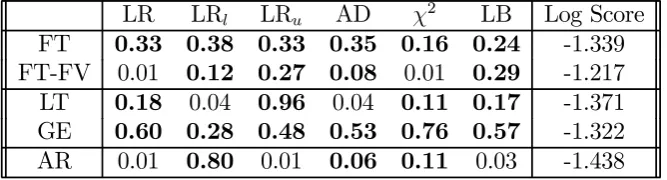
Examining the goodness of fit and independence pits tests presented in Table 1 (see Section 3.5.3 for discussion of the KLIC test), we see that the real-time inflation ensemble forecast densities, FT, based on the seven flexible trends are well calibrated at a 95% confidence level. (Instances of appropriate calibration are marked in boldface.13) The densities constructed using final vintage data, FT-FV, shown in the second row of Table 1 show evidence of calibration failure at 95% for two of thepits tests (LR and χ2).
11Given the large number of component densities under consideration in the ensemble, we do not allow for estimation uncertainty in the components when evaluating the pits. Corradi and Swanson (2006) reviewpits tests computationally feasible for smallN.
12When evaluating the density forecasts we treat them as primitives, and abstract from the method used to produce them. Amisano and Giacomini (2007) and Giacomini and White (2006) discuss more generally the limiting distribution of related test statistics.
Table 1: Ensemble Forecast Density Evaluation, 1991q3-2007q2
LR LRl LRu AD χ2 LB Log Score
FT 0.33 0.38 0.33 0.35 0.16 0.24 -1.339
FT-FV 0.01 0.12 0.27 0.08 0.01 0.29 -1.217
LT 0.18 0.04 0.96 0.04 0.11 0.17 -1.371
GE 0.60 0.28 0.48 0.53 0.76 0.57 -1.322
AR 0.01 0.80 0.01 0.06 0.11 0.03 -1.438
Notes: FV denotes final vintage data are used. LR is the p-value for the Likelihood Ra-tio test of zero mean, unit variance and zero first order autocorrelation of the inverse normal cumulative distribution function transformed pits, with a maintained assumption of normality for the transformed pits; LRu is the p-value for the LR test of zero mean and unit variance
focusing on the 10 percent upper tail; LRl is the p-value for the LR test of zero mean and
unit variance focusing on the 10 percent lower tail; AD is the small-sample (simulated) p-value from the Anderson-Darling test for uniformity of the pits assuming independence of the pits.
χ2 is the p-value for the Pearson chi-squared test of uniformity of the pits histogram in eight equiprobable classes. LB is thep-value from a Ljung-Box test for independence of thepitsbased on autocorrelation coefficients up to four. Log Score is the average logarithmic score over the evaluation period. The GE statistics are computed over a shorter evaluation period, reflecting the need for an extra training period (here set to 10 quarters).
3.5.3 Grand Ensemble and Benchmark
Mindful of the debate in the literature about the importance of linear output trends for forecasting inflation in real time, in the third row of Table 1 we report pits tests for the linear trend ensemble, LT. We also provide, in the fourth row, the tests for the grand ensemble, GE, based on the real-time combination of FT and LT variants.14 Thefinal row evaluates the forecast density from a simple benchmark AR(1) specification for inflation. The linear time trend variant, LT, and the AR(1) benchmark both fail to match the performance of the FT ensemble. The LT ensemble fails two of the sixpits tests, and the AR benchmark fails three of the six tests, at the (individual) 95 percent confidence level. For the AR, failure is marked for the independence component (picked up by LR and LB) of thepitstests. This is consistent with the view that the AR conditions on an incomplete information set by ignoring the output gap; see Corradi and Swanson (2006) and Mitchell and Wallis (2009). Moreover, the AR density is rejected in favor of either ensemble (FT or LT) using the KLIC-based test at a 95% confidence level, thereby indicating that the improvements observed in the log scores for the ensembles over the AR, reported in the
final column of Table 1, are statistically significant.
This result is noteworthy given the “perceived wisdom” in the macro forecasting lit-erature that parsimonious autoregressive specifications are “hard to beat”; e.g., see Stock and Watson (2007). This view relates to measures of point forecast accuracy in general, and RMSFE in particular.15 When examining the whole forecast density, AR models are easier to beat. We also examined (but do not report) AR benchmarks with lag order 2,3 and 4, with no qualitative differences in the results.
Turning to the grand ensemble, GE, we see that the real-time forecast densities are well calibrated for inflation. The performance of the GE is unsurprising given that FT ensemble performs well. However, consideration of linear time trends substantially alters the implied forecast densities for the output gap. Figure 4 provides a plot of GE predictive densities through our evaluation period. As with Figure 3 (the FT case), areas of highest mass are marked in white, and lowest mass in black. The GE results in multi-modal forecast densities with predominately two peaks stemming from the LT and FT ensembles. The LT gives predictive densities that almost always predict output below trend. Hence, where the FT ensemble predicts a boom, the LT ensemble typically indicates a slump. Even when the two peaks are relatively close, in 2000 and 2001, differences remain. Figure 5 provides the GE forecast density for an individual observation, 2000q1, as an example. As afinal robustness check, we repeated our grand ensemble exercise including the AR benchmark. In this case, we found the same broad story: the GE was well calibrated with no pits test failures for inflation. But the forecast densities for the output gap revealed strong multi-modality.
4
Conclusions
In this paper, we have proposed a methodology for producing predictive densities for the output gap in real time using a large number of vector autoregessions. Ensemble combination via a linear mixture of experts framework produces potentially non-Gaussian densities for the unobserved output gap. In our US application, the resulting ensemble produced well-calibrated forecast densities for inflation in real time, in contrast to those from simple univariate autoregressions which ignored the contribution of the output gap. We have also shown that data revisions altered our probabilistic assessments of the output gap based on univariate flexible trends. Adding linear detrending specifications via our grand ensemble indicated strong multi-modality for the unobserved output gap. The twin peaks associated with linear time trends and moreflexible trends, at times, pointed to output gaps of opposite sign. These issues are not apparent from more conventional assessments of the output gap. In future work, we plan to analyze monetary policy issues in an incomplete model space. We feel that a consideration of the contributions of data uncertainty to policy errors in the presence of multi-modal output gap nowcasts is warranted.
References
[1] Amisano, G. and R. Giacomini (2007), “Comparing Density Forecasts via Likelihood Ratio Tests”, Journal of Business and Economic Statistics, 25, 2, 177-190.
[2] Bao, Y., T-H. Lee and B. Saltoglu (2007), “Comparing Density Forecast Models”, Journal of Forecasting, 26, 203-225. First circulated as “A test for density forecast comparison with applications to risk management”, University of California, River-side, 2004.
[3] Baxter, M, and R.G. King (1999), “Measuring Business Cycles: Approximate Band-Pass Filters for Economic Time Series”, Review of Economics and Statistics, 81, 594-607.
[4] Berkowitz, J. (2001), “Testing Density Forecasts, with Applications to Risk Manage-ment”, Journal of Business and Economic Statistics, 19, 465-474.
[5] Beveridge, S., and C.R. Nelson (1981), “A New Approach to Decomposition of Time Series into Permanent and Transitory Components with Particular Attention to Mea-surements of the Buinsess Cycle”, Journal of Monetary Economics, 7, 151-174. [6] Canova, F. (1998), “Detrending and Business Cycle Facts”, Journal of Monetary
Economics, 41, 475-512.
[7] Carvalho, A.X. and M.A. Tanner (2006), “Modeling Nonlinearities with Mixtures-of-experts of Time Series”, International Journal of Mathematics and Mathematical Sciences, 9, 1-22.
[8] Christiano, L. and T.J. Fitzgerald (2003), “The Band Pass Filter”, International Economic Review, 44, 2, 435-465.
[9] Clark, T.E. and M.W. McCracken (2009), “Averaging Forecasts from VARs with Uncertain Instabilities”,Journal of Applied Econometrics, forthcoming. Available as Federal Reserve Bank of Kansas City Working Paper 06-12.
[10] Corradi, V., A. Fernandez and N.R. Swanson (2009), “Information in the Revision Process of Real-Time Data”,Journal of Business and Economic Statistics, forthcom-ing.
[11] Corradi, V. and N.R. Swanson (2006), “Predictive Density Evaluation”, G. El-liot, C.W.J. Granger and A. Timmermann, eds, Handbook of Economic Forecasting, North-Holland, 197-284.
[12] Croushore, D. and T. Stark (2001), “A Real-time Data Set for Macroeconomists”, Journal of Econometrics, 105, 111-130.
[14] Diebold, F.X., T.A. Gunther and A.S. Tay (1998), “Evaluating Density Forecasts; with applications tofinancial risk management”,International Economic Review,39, 863-83.
[15] Garratt, A., Lee, K., Mise, E. and K. Shields (2008), “Real-Time Representations of the Output Gap”, Review of Economics and Statistics, 90(4), 792-804.
[16] Garratt, A., G. Koop, E. Mise and S.P. Vahey (2009), “Real-Time Prediction with UK Monetary Aggregates in the Presence of Model Uncertainty”,Journal of Business and Economic Statistics, forthcoming.
[17] Genest, C. and K.J. McConway (1990), “Allocating the Weights in the Linear Opin-ion Pool”, Journal of Forecasting, 9, 53—73.
[18] Genest, C. and J. Zidek (1986), “Combining Probability Distributions: a critique and an annotated bibliography”, Statistical Science, 1, 114—135.
[19] Geweke, J. (2009),Complete and Incomplete Econometric Models, Princeton Univer-sity Press, forthcoming.
[20] Giacomini, R. and H. White (2006), “Tests of Conditional Predictive Ability”, Econo-metrica, 74, 1545-1578.
[21] Hall, S.G. and J. Mitchell (2007), “Density Forecast Combination”, International Journal of Forecasting, 23, 1-13.
[22] Hodrick, R. and E. Prescott (1997), “Post-War U.S. Business Cycles: An Empirical Investigation”, Journal of Money, Banking and Credit, 29, 1-16.
[23] Jore, A. S., J. Mitchell and S.P. Vahey (2009), “Combining Forecast Densities from VARs with Uncertain Instabilities”, Journal of Applied Econometrics, forthcoming. [24] Kascha, C. and F. Ravazzolo (2009), “Combining Inflation Density Forecasts”,
Jour-nal of Forecasting, forthcoming.
[25] Koop, G. (2003),Bayesian Econometrics, John Wiley.
[26] Laubach, T. and J.C. Williams (2003), “Measuring the Natural Rate of Interest”, Review of Economics and Statistics, 85, 1063-1070.
[27] Lindley, D. (1983), “Reconciliation of Probability Distributions”, Operations Re-search, 31, 866—880.
[29] Marcellino, M., J. Stock and M.W. Watson (2003), “A Comparison of Direct and Iterated AR Methods for Forecasting Macroeconomic Series h-steps Ahead”,Journal of Econometrics, 135, 499-526.
[30] Mise, E., T-H. Kim and P. Newbold (2005), “On the Sub-Optimality of the Hodrick-Prescott Filter”, Journal of Macroeconomics, 27, 1, 53-67.
[31] Mitchell, J. and S.G. Hall (2005), “Evaluating, Comparing and Combining Density Forecasts Using the KLIC with an Application to the Bank of England and NIESR “Fan” Charts of Inflation”,Oxford Bulletin of Economics and Statistics, 67, 995-1033. [32] Mitchell, J. and K. F. Wallis (2009), “Evaluating Density Forecasts: Forecast Combi-nations, Model Mixtures, Calibration and Sharpness”, NIESR Discussion Paper No. 320.
[33] Molteni, F., R. Buizza, T.N. Palmer and T. Petroliagis (1996), “The New ECMWF Ensemble Prediction System: methodology and validation”,Quarterly Journal of the Royal Meteorological Society, 122, 73-119.
[34] Morley, J.C., C.R. Nelson and E. Zivot (2003), “Why Are the Beveridge-Nelson and Unobserved Components Decompositions of GDP so Different? Review of Economics and Statistics, 85, 235-243.
[35] Morley, J. and J. Piger (2009), “The Asymmetric Business Cycle”, Washington Uni-versity in St. Louis, unpublished manuscript.
[36] Morris, P.A. (1974), “Decision Analysis Expert Use”,Management Science, 20, 1233-1241.
[37] Morris, P.A. (1977), “Combining Expert Judgments: A Bayesian approach”, Man-agement Science, 23, 679-693.
[38] Noceti, P., J. Smith and S. Hodges (2003), “An Evaluation of Tests of Distributional Forecasts”,Journal of Forecasting, 22, 447-455.
[39] Orphanides, A. and S. van Norden (2002) ,“The Unreliability of Output-Gap Esti-mates in Real Time”, Review of Economics and Statistics, 84, 4, 569-583.
[40] Orphanides, A. and S. van Norden (2005), “The Reliability of Inflation Forecasts Based on Output-Gap Estimates in Real Time”,Journal of Money Credit and Bank-ing, 37, 3, 583-601.
[41] Raftery, A.E., T. Gneiting, F. Balabdaoui and M. Polakowski, (2005), “Using Bayesian Model Averaging to Calibrate Forecast Ensembles”, Monthly Weather Re-view, 133, 1155—1174.
[43] Rudebusch, G.D. and L.E.O. Svensson (2002), “Eurosystem monetary targeting: lessons from US data”, European Economic Review, 46, 3, 417-442.
[44] Sims, C. (2008), “Inflation Expectations, Uncertainty, and Monetary Policy”, Prince-ton University, unpublished manuscript, http://sims.princePrince-ton.edu/yftp/BIS608/
[45] Stock, J.H. and Watson, M.W. (1999). “Forecasting Inßation”,Journal of Monetary Economics 44, pp. 293-335.
[46] Stock, J.H. and M.W. Watson (2007), “Has Inflation Become Harder to Forecast?”, Journal of Money, Credit, and Banking, 39, 3-34.
[47] Timmermann, A. (2006), “Forecast Combination”, G. Elliot, C.W.J. Granger and A. Timmermann, eds, Handbook of Economic Forecasting, North-Holland, 197-284. [48] Wallis, K.F. (2003), “Chi-squared Tests of Interval and Density Forecasts, and the
Bank of England’s fan charts”, International Journal of Forecasting, 19, 165-175. [49] Wallis, K.F. (2005), “Combining Density and Interval Forecasts: a Modest Proposal”,
Oxford Bulletin of Economics and Statistics, 67, 983-994.
[50] Watson, M.W. (1986), “Univariate Detrending Methods with Stochastic Trends,” Journal of Monetary Economics, 18, 49-75.
[51] Watson, M.W. (2007), “How Accurate are Real-Time Estimates of Output Trends and Gaps?”, Federal Reserve Bank of Richmond Economic Quarterly, Spring 2007. [52] Winkler, R.L. (1981), “Combining Probability Distributions from Dependent
-3 -2 -1 0 1 2 3 4
Figure 1: Output Gaps, Various Flexible Trends, Final Vintage
0.1 0.2 0.3 0.4 0.5 0.6 0.7 0.8 0.9 1
Figure 2: One Step Ahead Probability of a Negative Output Gap, Flexible Trend Ensemble
0 0.05 0.1 0.15 0.2 0.25 0.3 0.35