The Stochastic Model for «Shnoll Effect»

The Stochastic Model for «Shnoll Effect»

V. A. Meshkoff

Chaotic Modeling and Simulation International (CMSIM), Section Chaos in Astronomy and Astrophysics, Europe, Republic Crimea, Russian Federation

Copyright©2017 by authors, all rights reserved. Authors agree that this article remains permanently open access under the terms of the Creative Commons Attribution License 4.0 International License

Abstract

«Shnoll effect» proved to be at the histograms study of a wide variety of processes. This paper examines the effect mainly for the examples of radioactive decay and chemical reactions. S.E. Shnoll supposed that the observed processes are caused by unknown Cosmophysical effects. In this article, we suggested not only a qualitative explanation of the effect, but also its mathematical model. It allows to get some quantitative estimation and to optimize the process of observation and data handling. To this end, we developed a quantitative method of estimation «similarity of histograms» that allows the use of standard computer programs. As far as «Shnoll effect» at present is not currently recognized by the scientific community, we suppose that the use of mathematical model and adequate methods of data handling allow synonymously solving that problem.

Keywords

Shnoll Effect, Radioactive Decay, Histogram, Fluctuation, Random Variables, White Noise, Deterministic Effects, The Poisson Distribution, The Binomial Distribution

1. Introduction

The «Shnoll effect» is revealed in the study histograms for the various processes [1, 2]. Further we will mainly focus on the researching of the processes of radioactive decay. Then there is S – Source of decay particles, in particular, α

-particles; C – Particle Counter with recording equipment. A particle gets into C, create corresponding response, recorded as a single signal (pulse). Private signal of C output corresponds to the number of pulses per time T. Since usually only the number of pulses is counted, the signal can be represented as

1

(

)

M

( , , )

_i

i

X t MT

x i T n

=

=

=

∑

(1)

Here the private signal

x i T n

( , , )

_i means that for the time interval

iT i

− −

( 1)

T T

=

there are

n

_i pulses registered. The set of such signals in the time

MT

is the experimental

information about the process of radioactive decay. This information is presented in the form of histograms, step function

[ ( )]

( )

Hist X t

=

H n

(2) where

H n

( )

– number of private signals containing

n

pulses.

To study the «Shnoll effect» (SE) it is recorded some number

S

of such sequential histograms in time

SMT

. Further, these histograms can be summed, averaged, or compared at the «similarity» of its shapes.

2. Stochastic Description of Radioactive

Decay

Since at this approach the arraignment of pulses in time does not value, may be even to assume that in the particular signal pulses are uniformly distributed. If (1) corresponds to the accurate recording of the particles, it is generally believed that for the process of radioactive decay values

( )

H n

correspond to a Poisson distribution [3].

(

)

!

n

N T n

N T

e

n

λ

λ

ω

₌

− ₍₃₎

where

ω

_n – the probability of detecting

n

particles in a time

T

,

N

– the number of radioactive atoms in S,

λ

– speed of particle radiation. In this case, the average value

av

n n

=

determined from histograms corresponds to a value av

n

=

N T

λ

, and determine by period of half-decay (from reference) value

λ

, may be to estimate the effective value of the number of radioactive atoms in S.

av

eff

n

N

T

λ

=

(4)

It is the question of interest whether two or more atoms of

S can emit particles at the same time, or there is a finite amount of time between these events?

of the pulse and the minimal allowable time between pulses, the counter dead time. Possible counters errors [4] further will be neglected. In this case for the «right» counter C there are some permissible values

max

,

/

per

n

r T

τ

=

τ

= ≅

τ

(5)

Then will be assume that there are no coincidences of pulses, and any time interval

T

in relation to the particular signal at the input C may be regarded as consisting of

r

cells.

For each such cell with a constant probability

p

pulse or is in it («success»), or with the probability

1

−

p

is not («failure»). So we have corresponding with Bernoulli testing scheme [5].

The probability that there will be

n

successes in

r

testing

(

)

( ; , )

n n

1

r n

r

n r p

C p

p

ω

−

=

−

(6)

If

r

is sufficiently large and

p

is sufficiently small, an average value is

n

_av

=

rp

. For large

r

from binomial distribution (6) follow classical Poisson approximation

( )

!

n

rp n

rp

e

n

ω

₌

− ₍₇₎

The correspondence between (3) and (7) would be in that case if equate the values

n

_av. Then

,

N T

N T rp

p

N

r

λ

λ

=

=

=

λτ

(8)

Since, by definition

p

≤

1

, then from (8) we find the necessary requirements for the C, i.e. for the resolution capacity of counter, corresponding to the properties of the applied source S

1

N

τ

λ

≤

(9) That result corresponds to some condition of S, when particle radiation is sufficiently rare event for right Poisson probability (7), (8). We find that the temporal characteristics of the meter must be coordinated with the specific source of the particles.

It is believed that for any moment of time the radioactive decay is equally probable [3]. With reference to the counter, this means that all periods

T

are equal, and if the period divided into some number

r

of identical intervals (cells), then for sufficiently large observation time, the pulses that get into these cells will be evenly distributed.

3. Microscopic and Macroscopic

Fluctuations

There are many stochastic processes that can be described with use of a similar scheme. It is known that a simple

random walk model, based on the binomial distribution, similar to (6) leads to the relations, correctly described the process of diffusion and Brownian motion. It turns out that a similar scheme of reasoning is applicable to many phenomena in physics and another field of science, in cases where relatively slow observed fluctuations of the system states are the result of a huge number of small random unobserved effects [6].

These effects in specific cases may be collisions of atoms and molecules, their thermal vibrations, noise and fluctuations of electromagnetic nature, etc.

We come to realization that the observed fluctuations of the stochastic nature are a consequence of the influence of unobservable (microscopic?) fluctuations of different nature. Further assume, without proof that in nature there is a corresponding universal principle: Any observable stochastic physical processes occur as a result of microscopic

unobservable stochastic fluctuations. This means that it is

not for random process any description, except probable, because if we were able to control the causes of random behavior of a physical system, the process would cease to be accidental.

Note that for throwing coin and observation occurring of «heads» or «tails», we cannot control all the causes of a particular outcome, even if they are not microscopic for a concrete coin. Otherwise, the coin becomes «wrong», i.e. predictable.

From the point of view of mathematical formalism, we have three levels of description of stochastic processes. Discrete Level 1 is characterized by the Binomial distribution, and for the continuous speed of the process it transforms into a discrete Level 2 – Poisson distribution, and then it is the transition from discrete to continuous variables – Binomial and Poisson distributions are transformed into Level 3 – Gaussian distribution (law of large numbers) [5].

As returning to radioactive decay then we consider it from the point of view of the universal principle accepted above. In nuclear physics it is believed that for separate atom or isotope radioactive decay happens spontaneously, «the phenomenon of radioactivity consists in spontaneous disintegration of atomic nucleus with emission of one or several particles» [3]. It is established that radioactivity is the quantum mechanical phenomenon caused by electromagnetic, strong and weak interactions of particles in a nucleus. Atoms and their nucleus are complicate dynamic, but not static systems. Without going into the further details, we will notice that in such dynamic systems it is inevitable existence of microscopic unobservable fluctuations, in that case of quantum character.

Therefore it is reasonable that we can refine the definition,

– the phenomenon of radioactivity is the decay of nucleus

under the influence of quantum fluctuations with the

emission of one or more particles. Nothing prevents us to

In textbooks on nuclear physics it is also claimed that «essential property of the phenomenon of radioactivity is independence of a constant of disintegration

λ

of time» [3]. However from SE follows that it, at least, not always so and there are phenomena when this independence is broken. In this case it is necessary to consider, taking into account the universal principle that value

E

₀doesn't depend on time.

4. Shnoll Effect and its Qualitative

Considerations

Thus, from the point of view of orthodox nuclear physics influence on quantum fluctuations of atoms is impossible, but SE is affirmed the inverse. Therefore we will assume further that under some conditions such influences happen, and for that reason the observed process differs from usual «Poisson».

For simplification we will consider further that the source contains radioactive atoms only of one sort, there are removed hardware errors and the outside physical phenomena, for example, an influence of space radiation and so on.

By the way noted that the physical properties of the sources may be different, – most obvious difference, for instance, is that they may be gaseous, amorphous or solid. From qualitative considerations it is believed that in the first two cases, the decay conditions must be similar to the decay conditions of independent atoms under the influence of quantum fluctuations inside the nucleus. In that case, the effect of external influences is believed likely minimal.

In the case of solid-state sources the radioactive atoms are no longer independent, and quantum fluctuations are distributed throughout the volume of the source. Thus sizably increasing the amount of space, in which external influences can contribute. In the present case, we will not put forward suppositions about their nature. Just out of qualitative considerations it is follow that may be the physical conditions when into the source is interaction of quantum fluctuations and external, for example, «cosmos-physical factors».

Further naturally to assume that the external influences and internal fluctuations can either are in phase or in anti-phase, and on that dependence the rate of decay will either increase or decrease. That allows giving a reasonable explanation of the experimentally observed in SE oscillating «fine» effects, revealed in the histograms [1, 2].

It is easy to show that in the same way, i.e. by interaction «external signal» with internal fluctuations of radioactive sources, explains all the observed effects in experiments of Shnoll and collaborators.

Non-randomness of the «fine» structure of histograms shape in measurements of different nature [1]: observed histograms «poly-extremality» do not disappear with the growth of the number of measurements, i.e. there are additional peaks and gaps that are not in the Poisson

distribution.

This is explained by the interaction of internal fluctuations with «external signal», having in general case the random and deterministic (systematic) components. In result there may be observed not only the «fine structure», but significant deviations from the Poisson distribution. The critics of Shnoll [8] at this correctly pay attention: dispersions and distribution shape, obtained experimentally in [1], are significantly different. In one instance, the dispersion decreases, the distribution peak increased compared to Poisson distribution (Figures 1 and 2 in [8]), but in another case there is the reverse – the dispersion increases, the peak decreases (Figure 5 in [8]).

However, within the limits of our model, this means in first case there are internal fluctuations in phase with the «external signal», and in second case – in anti-phase.

Note that without a concrete model for the observed effects, there are confused explanations in [2]. On the one side, they state that «there is no doubt in the submission of the radioactive decay to Poisson statistics», but further they state, that «regardless of the reasons of some deviations <...> from the Poisson distribution it is not due to the histograms fine structure».

In the proposed model, by contrast, the deviations from «Poisson» and «fine structure» in general are interconnected and have the «external signal» as the cause.

Uncasual repetition of histograms shape in time [1]: it is found out that the repetitions of the same shape in a series of successive histograms are most likely in the nearest neighbor time interval. Furthermore, the similarity of histograms shape is detected with periods 24 hours, 27 and 365 days. From all the totality of the data concludes about the impact of cosmos-physical factors.

In our model, this property is easily explained by the deterministic nature of the «external signal», interacting with internal fluctuations of the particle source. It is likely that the source of this «external signal» is the Sun, with the Earth's rotation and the positions of the Moon.

At the same time, critics [8] note that Shnoll and collaborators do not have a quantitative method of comparing the «similarity» of histograms, using based on visual analysis method that contain a significant subjective moment.

Synchronization of realization of histograms shapes in the processes of different nature [1]: it is detected by simultaneous independent measurements conducted at a distance, and even in the far-located geographical points.

Again, this is easily explained in limits of our model: it means that the deterministic component of the «external signal» render a similar synchronizing effect on the stochastic processes of different nature in different geographical locations, interacting in each case with internal fluctuations.

The randomization of the initial time series according to standard criteria [1]: Shnoll and collaborators manifest that the connection between the histograms and the «conformity with a laws of the motion of the studied processes in time <...> traditional methods <...> failed to expose». They assert that «the process of radioactive decay is completely random – it is „white noise“».

In terms of our model, this means that by using the counter

C, with period of counts

T

, in the distinguishable

r

time cells will be on the average registered almost the same number of pulses. The distribution all over the cells averaged over a large period of time would be equally probable, which corresponds to the binomial distribution, transitional to Poisson, and then to Gaussian.

Again, our model can give a qualitative explanation of this effect. Assume that «external signal» has a noise component and deterministic oscillating component, for example, some superposition of sinusoidal oscillations. In a result of the interaction this signal with internal fluctuations of source S

will occurred some change in the intensity of «white noise» that correspond to acceleration of the process of radioactive decay or its deceleration.

Periods of sinusoidal oscillations of «external signal» may not coincide with the period of counts

T

, then at the time averaging none deviations to be detected from equally probable distribution of pulses at cells. Thus, we find the explanation for the seemingly strange assertion [2] that the «fine structure» of histograms does not depend from the reasons of deviation from Poisson distribution.

Indeed, as we have seen above, for an explanation of the results [1, 2] it is appropriate to assume that the «external signal» can increase or decrease dispersion of the radioactive decay process in comparison with the dispersion of corresponding Poisson process. But the «fine structure» due to the presence deterministic oscillatory component in «external signal», and it is in principle can occur even with a constant average dispersion of radioactive decay!

The negative correlation «the results scatter» with solar activity [1]: it is indirect evidence of «external signal» effects. Rather, it means that the result of the interaction of internal fluctuations with a deterministic component of the «external signal» in most cases is not symmetrical. This effect is known in statistical radio-physics [10, 11].

Thus, we conclude that in the framework of the proposed stochastic model naturally receive explanation of all the main experimental results Shnoll and employees set out in [1, 2]. This model is, for this reason, should be applicable not only to radioactivity but also to all processes mentioned in [1]. «External signal/effect», characteristics and nature of which we will not discuss here, must in all cases originate from the same source with the identical timing characteristics on a large geographical area.

Accordingly, we can determine the Shnoll effect: The changeability and synchronization of probabilistic characteristics of stochastic processes as a result of «external influences», presumably of cosmos-physical origin.

5. Additional Considerations

Adduce some additional considerations that external impact SE has deterministic and periodical character. In general case

λ

is not constant, but cannot be monotonically increasing (otherwise

n

_avincreases with time), and then instead of (3) we have

(

)

0

,

( )

!

n _T

N n

N

e

t dt

n

µ

µ

ω

₌

−

µ

₌

λ

∫

(10) Deviations from the Poisson process can be explained if for each particular signal

x i T n

( , , )

_i there will be its parameters

( 1)

( )

iT

i i T

t dt

µ

λ

−

=

_∫

(11)

According to (11) we can have a few discrete values

µ

_k, and a histogram (2) will be determined as the superposition (mixture) of several Poisson processes, which, in principle, and can give the «fine structure» of the experimental histograms.

For establishing the adequacy of the proposed model, it is easy to suggest an appropriate physical model for reproduction of our SE model properties. For example, it may be a pulse generator in the standby mode (waiting regime), generating the pulse under the influence of fluctuations in a trigger circuit, and then returning to the initial state. «External effects» can be simulated by supplying additional noise or periodic signal in the trigger circuit.

Also, as simple physical model can serve electronic devices with the shot noise, that obeys Poisson distribution. It is sufficient to consider the vacuum triode in regime of small shot currents. Suppose that during the time

T

it is possible to detect the arrival on the anode each of the electrons like at the experiment with alpha particles discussed above. If now give periodic potential on the triode grid, it will modulate the shot current, simulating a real stochastic model SE. Its properties are possible to study experimentally by varying the «external influence».

However, there are publications [8], stated that the effects which existence claim Shnoll and collaborators, are not observed. But, the analysis of such publications shows that usually they refer to experiments with significant differences from those criticized.

Restricted only radioactive decay processes, for example, we see that the experiment with the preparation 55

Fe

[1] is opposed to the experiment with the same preparation [8], but deviations from Poisson distribution and «fine structure» of histograms are not observed. However, about coincidence of all experimental conditions in both cases according to the publications it is problematic to judge.

is opposed similar experiment with the preparation 241

Am

[8], where again did not find signs of SE. There are other such publications, where the SE is denied on the basis of private experiments and different assumptions about the fallibility of Shnoll with collaborators observations. On the other hand decennials of observations and of huge accumulated experimental material allows experienced scientists claim about proof «theorem of the existence» for effect that many opponents or may be most of the scientific world, is still, at best, considered hypothetical.

One of the reasons for this contradiction is that the conditions for SE observing are not defined in [1, 2] with exhaustive plentitude. The authors do not give the «recipe», the maintenance of which will allow others experimenters with the confidence to reproduce this effect. Moreover, judging by some of the private statements and publications, the authors believe that the effect should be observed almost «always and everywhere» for «good» experimenter. With above accounted, it is difficult to accept.

Therefore, the «existence theorem» should be supplemented with «necessary and sufficient conditions», ensuring the reproduction of the effect.

From this viewpoint, the most perspective are experiments with radioactive solid preparations under condition with

direct registration of positive charged α-particles counter. In this case at the output of the counter should be impulse of

definite shape, which allows not only fixing the α-particles, but also reliably distinguishing these pulses against background of various disturbances, including other pulses with other forms. In this case, it will be possible to completely eliminate the assumption of critics about possible mistakes and errors of experiments.

It is concerned the cases when α-decay fix in indirect way by registration concomitant X-ray radiation or γ-quanta. There need thorough analysis of all registration process and its trustworthiness, that from publications [1, 2, 9] not displayed.

Another possibility for removal of contradictions consist in complete using of information, that may be get in

experiments on radioactive decay with α-particles registration. In present it is possibilities for recording complete signal

X t

( )

at output C on electronic storage device. This signal in ideal has presentation as secession of identical pulses and its timing arrangement, i.e. has view

( )

(

)

X t

F t t

ν ν

=

∑

−

, where

F t

( )

characterizes form of

pulses with small duration

∆ <

τ τ

_per . Practically it is sufficiently to registration and recording all values

t

ν ,

connected with any characteristic point of pulses.

From publications [1, 2] and analogical it is vague if that information records and use in full measure. With aid of computer methods and program processing the recorded signal may be repeatedly to use for receiving knowledge about concrete realization of radioactive decay process and its difference from Poisson process.

6. Appendix

6.1. Simplest Physical Model for Shnoll Effect

Look at some system (source), where under influence of internal fluctuations (noises) occurs observed macroscopic events, for example, radioactive decay and flying out

α-particle, pulse generation of flip-flop scheme, and so on. Assume, that such event occur every time when energy of fluctuations exceed some threshold value

E

₀.

Similar problem examine in statistical radio-technique [10, 11]. In our case will suppose that fluctuations describe by realizations

y t

( )

of stochastic process

Y t

( )

. Observed event occur when

y t

( )

crosses threshold value

E

₀ «from down upwards». It named as positive overshoot

Y t

( )

on level

E

₀.

Suppose that

Y t

( )

is stationary and continuous, then possible to select such interval

∆

t

, that in limits of this interval it will be not any positive overshoot, or it will be only one.

Sole positive overshoot occur if: 1)

y t

( )

<

E

₀ , 2)

0

(

)

y t

+ ∆ >

t

E

.

Suppose that for realizations

y t

( )

of stochastic process may be to determinate the derivative, then

(

)

( )

y t

+ ∆ ≈

t

y t

+ ∆

y t

′

and get conditions for realization of positive overshoot

0 0

0,

( )

y

′

≥

E

− ∆ <

y t y t

′

<

E

For further decision assume that it is known joint distribution

p y y

( , )

′

and then for overshoot probability get

0

0

0

0 0

( , )

E

( , )

E y t

P

∞

p y y

dydy

t p E y y dy

∞

′ − ∆

′

′

′ ′ ′

∆ =

_∫

_∫

≈∆

_∫

(A.1) Average value of overshoot by time unit determinate as

0 0

0

( )

E

P

p E y y dy

( , )

t

λ

=

∆

=

∞

′ ′ ′

∆

∫

(A.2)

In simplest case

y t

( )

and

y t

′

( )

are statistically independent (as example, for Gaussian processes [10,11]), and then

p y y

( , )

′

=

p y p y

₁

( ) ( )

₂

′

, so from (A.2) follow

0 1 0 2 0

( )

E

p E

( )

p y y dy

( )

λ

=

∞

_∫

′ ′ ′

(A.3)

corresponding change of the threshold value, which will now of the time depend, i.e.

E t

( )

=

E

₀

+

f

_t. We will confine to the case of a continuous function

f

_t

=

f t

( )

whose variations in time

∆

t

are negligibly small. Then the previous presentation (A.3) remains valid for replacing

0

( )

E

→

E t

. As a result, we have

1 0 2 1

0

( )

t

p E

(

f

_t

)

p y y dy

( )

_f

F t

( )

λ

=

+

∞

∫

′ ′ ′

= +

λ λ

(A.4),

where

λ

₁– the constant component of the periodic function

( )

t

λ

, and

λ

_f– the scale factor of the normalized periodic function

F t

( )

with period

Ψ

, which does not have a constant component. In general case it is convenient to normalize an area under the curve

F t

( )

during the half-period

/ 2 / 2

0 0

( ) ( ) , ( ) ( ) 0, ( ) ( ) 0

F t dt F t dt F t F t F t F t

Ψ Ψ

+ = − = Ψ + = > − = <

∫

∫

Returning to relations (10), (11) and to the conditions of Shnoll experiment, we have with account of (A.4)

1 1

0 0 0

( )

(

( )

( )

T T T

f f

t dt

F t dt

T

F t dt

µ

=

_∫

λ

=

_∫

λ λ

+

=

λ

+

λ

_∫

(A.5) If periods coincide, i.e.

T

= Ψ

, then from (A.5) for this case

µ λ

=

₁

T

. The process will be perceived as a stationary Poisson process with the distribution (3), where the standard value

λ λ

≠

₁. No «fine structure» will be registered.

Let us consider the cases when

T K

= Ψ

,

K

≥

0

. Then for case of an arbitrary value we have

[ ]

{ }

,

[ ]

,

[ ]

{ }

K

=

K

+

K

= +

k

χ

k

=

K

χ

= −

K

K

=

K

, where the fractional part of the number

K

is positive, i.e.

0

< <

χ

1

. So

0 0 0

( )

k

( )

( )

T

F t dt

χ

F t dt

χ

F t dt

Ψ+ Ψ Ψ

=

=

∫

∫

∫

For an arbitrary value

K

, we calculate the partial values

( )

( )

( 1) ( 1) ( 1) 0

( ) i k ( ) i ( ) ( ( 1) )

iT

i T i k i

F t dt χ F t dt χ F t dt χ F t i dt

χ χ

χ

Ψ+ Ψ Ψ Ψ

− − Ψ+ Ψ − Ψ

= = = + − Ψ

∫

∫

∫

∫

(A.6)

It is obvious that the extremely values for the right-hand side of (A.6) are possible only when

χ

=

1_{2, as a result, we}

get

/ 2

0

,

( ( 1) / 2)

,

i odd

F t i

dt

i even

Ψ

_

_{Ψ −}

+ − Ψ

_{= }

−Ψ −



∫

(A.7)

Although this integral is independent of 1 2

K

= +

к

, it follows from (A.5) that the constant component

λ

₁

T

practically will dominate at sufficiently large

K

:

1₂

1

T

f

(

1 k f

)

T

λ

µ λ

=

+ Ψ =

λ

λ

±

₊

The greatest contribution of «external influence» will be at

1₂

0,

k

=

T

= Ψ

.

Taking into account the relations (A.5), (A.6) and (A.7) we obtain in this case

1 1

1 ( 1)

(

2 ),

( )

(

2 ),

iT

f

i f

f i T

T

i odd

T

F t dt

T

i even

λ

λ

µ

λ

λ

λ

λ

−

+

−



=

+

_{= }

−

−



∫

(A.8) With respect to the Shnoll experiment with the realizations (1), this means that half of the realizations correspond to the Poisson process (3) c

λ

+

=

λ

₁

+

2

λ

f, and the other half to the Poisson process c

λ

−

= −

λ

₁

2

λ

f . As a result, the experimenter will receive a histogram approaching a mixture of two Poisson distributions.

It is known, the sum of two or more random variables with Poisson distributions again gives the Poisson distribution. A

mixture of two or more such random variables, under certain proportions, is fully capable of forming poly-extremely distributions. In the simplest case considered above

(

)

(

)

1

1

2

!

2

!

n n

N T N T

n

N T

N T

e

e

n

n

λ λ

λ

λ

ω

=

+ − +

+

− − − _(A.9)

The corresponding distributions for different ratios

1

f

λ λ

and

n N T

₁

=

λ

₁

=

100

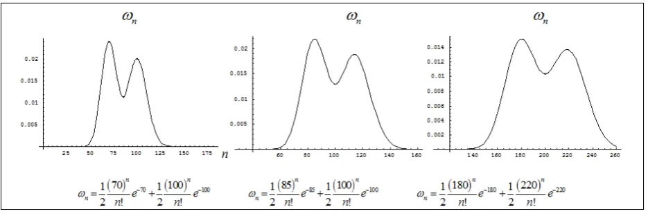
are shown at Fig. A1. 1-3. We get that in this variant Shnoll experiment is quite effective for detecting weak «external influences», or, equivalently, for weak external signals against a background of noises. Usually in radio-technique and radio-physics such a problem is posed for a signal-to-noise ratio of 1/1, and here we see that a «signal» can be detected at a ratio

1

0,05 0,075

f

[image:7.595.72.540.79.235.2]

Figure A1. 1-3. The distributions for different ratios

λ λ

_{f 1}and

n N T

₁

=

λ

₁

=

100

; ω_n

In general case, it is easy to see that «optimal reception» is possible when

K

=

0,

T

= Ψ

χ

, where 1

2

≤ <

χ

1

, is a

rational or irrational number. Accordingly, in the general case, for an arbitrary mixture of distributions, we obtain

(

)

_,

₁

!

j

n

j N T

n j j

N T

e

n

λ

λ

ω

₌

∑

β

−

∑

β

₌

(A.10)

For example, if 3 4

χ =

we obtain from the formulas (A.5), (A.6) and (A.10) the distribution with three vertices and two dips, etc.

It remains to consider the cases when

K

=

0,

T

= Ψ

χ

,

but 1

2

0

≤ <

χ

. In this case, the period of «external impact» exceeds or significantly exceeds the sampling period

T

, for example, becomes comparable with the time

MT

corresponding to obtaining of samples necessary for constructing the histogram. According to the formula (A.5), in this case for different samples we will have different values

µ

_i, and as a result, the histogram will again reflect the mixture of Poisson processes.

Thus, it is shown that we have the physical model reproducing the basic properties of the histograms obtained in Shnoll experiments.

If we now take into account that the actual «external effect» can have a complicated shape with many periodic components, noise components, quasi-periodic components of finite duration etc., then one can understand why in SE are observed histograms that deviate significantly from the classical Poisson process. Nevertheless, SE is based on the existence of deterministic external periodic effects, for which should exist an optimal method of observation.

6.2. Optimization of Shnoll Experiments

Considering the histograms given in [1, 2], one can see that they have a number of vertices and gaps exceeding the number of those at Fig. A1. 1-3. This means that the experimental conditions are not chosen in optimal way. In addition, «external influences» may have a more complex

character, compared with the deterministic periodic effects discussed above. It can relevant to quasi-deterministic signals [10, 11], i.e. has a random phase or amplitude, fluctuating waveform of signal. From our point of view, the Shnoll results indicate that there is an essential deterministic component, which within limits of the proposed model has a periodic character. Therefore, the optimal experiment should lead to histograms of distributions similar at Fig. A1. 1-3, in that will be possible to estimate the repetition period of the signal and the ratio

λ λ

_{f 1} . And since there are Shnoll reports on the direction of the effect [9], then it will be possible to obtain more detailed information about the «external effects».

Obviously, beforehand it is not possible to choose ratio

2

T

Ψ

=

, and then, at first glance, it is necessary to repeat the experiment at different

T

, approaching the optimal ratio. However, at present, this need can be avoided if, as mentioned above, the entire video signal at the output of the counter C is registered, digitized and recorded on electronic devices.

For example, in the case of experiments with radioactive alpha-decay, it is sufficient to record the time of appearance at the output C for each pulse, or the time interval between subsequent pulses. At the availability of such an array of data, there is no need to conduct multiple experiments to determine the optimal conditions and thus the parameters of the «external impact». It can be found using digital computer data processing techniques.

A computer program, using the same array of experimental data to construct histograms at different values

T

, will find the optimal ratio and will get estimation the signal parameters.

definite and efficient to register the «cosmos-physical factor» even if in experiments on radioactive decay, and the need for proofs of the «similarity» of the histograms of various processes will fall away, just as indirect evidence loses its significance in the presence of direct proof.

Another question of interest is the applicability in this case of existing methods for recognizing deterministic signals against a background of random noise. Judging by the statements of Shnoll, in this case these methods do not work. Indeed, if we turn to the methods of detecting and receiving signals against a noise background [10, 11], then an analogy with the Shnoll experiment is not found. In this case, the signal as if is built into the noise, it is «inside» the noise, so select one or the other known method of optimal signal reception does not work. Correlation analysis for the noise signal is also ineffective. The author did not analyze the possibility of applying a new «standard» approach – wavelet-analysis conformably to the entire time series of data. But, judging by Shnoll's remark, this method is known to him, and apparently did not give anything.

Nevertheless, in addition to the discussed above, another method of detecting and distinguishing the «useful signal» from Poisson's «white noise» was found in the limits of the proposed stochastic model.

As already indicated in the derivation of formula (6), it is possible to divide the studying time interval

T

into

r

identical time cells. If the radioactive decay is a purely Poisson process, then under these conditions we have an equiprobability temporal distribution of the pulses at the output C in time cells, or for sufficiently large

r

0

,

T

1

d

d

d

T

τ τ

τ

ω τ

=

∫

ω τ

=

(A.11)

Under the conditions of the Shnoll experiment, taking into account (A.5), this distribution has no longer equiprobability

1

0

(

( ))

( )

_,

T

₁

f

F

d

d

d

d

τ τ

λ λ

τ

τ

λ τ τ

ω τ

ω τ

µ

µ

+

=

=

∫

=

(A.12) It is not difficult to see that when

λ

f

=

0

we return at

(A.11).

Having all the temporary information about the experiment, we can construct a histogram, using the partitioning of the interval

T

into

r

cells, i.e.

T r dτ

/

≈

.

Each realization

x i T n

( , , )

_i is considered as realization of a random process with period

T

and with a zero reference count of the position of the pulses.

This means that the corresponding computer program divides the entire experiment period

MT

into

M

identical periods with the

r

cells, and then presents a histogram

[ ]

[ ( ) / ; / ] ( , , )i , 1,...

i

T

Hist X t M T r H x i T n j H j j r

r

 

= _ ∈ _= =



∑



(A.13) For a Poisson process the histogram (A.13) must correspond to a uniform distribution.

Consider now the case corresponding

Ψ

T

=

2

and Fig. A1. 1-3. Paradoxically, at first glance, but there must be a uniform distribution or close to it!

In that affair half of the realizations give an increase in the «density» of the pulses during the positive half-cycle

F t

( )

, and the other half of the realizations gives on the average during the half-period the same decrease. As a result, the experimenter will receive a temporal histogram, practically corresponding to a uniform distribution.

The optimal option for the time histogram corresponds

1

T

Ψ

=

. In this case we obtain from (A.12)

1 1

1 1

1 0

( ) _{( ) 1}

1 ( ) ( ( ))

f f f

T f F F F T T F d τ

λ λ

τ

λ λ

τ

λ

ω

τ

λ

λ

λ λ

τ

τ

+ +   = = = _ + _   +

∫

(A.14) As a result, the histogram at Fig.A2.2 corresponding to (A.14) presents a uniform distribution, as if modulated by an «external effect». A paradox here is too! The histogram (2) at Fig.A2.1 corresponds to a purely Poisson process and to the distribution (3) with the parameter

λ λ

=

₁.

[image:9.595.75.539.81.260.2] [image:9.595.81.535.286.469.2]

Figure A2. 1-2. The histogram Poisson process (left) and it’s modulated temporal distribution

Figure A3.1. Graphic presentation for successive measurements of the chemical activity

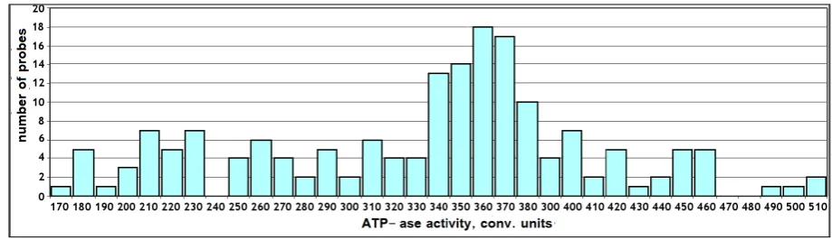
Figure A3.2. Histogram for chemical activity distribution

6.3. Modeling Distribution

The previous was written before acquaintance with the recently published book of S.E. Shnoll [12]. Unfortunately, it lacks at least one complete experimental data protocol, as well as the entire process of treatment the results of observations with using the chosen method and obtaining a concrete conclusion on this basis.

If the graphic characteristics of the 1957 experiment are

given (Figure 1, 2 of [12, p. 18]), then the protocol of this experiment that can be processed either by known methods of mathematical statistics or with the help of the above approach is not given. Nevertheless, already from this material it is possible to draw some conclusions, on the basis of the proposed model.

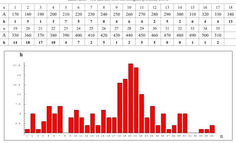
[image:9.595.73.533.495.628.2]

[image:10.595.65.544.85.375.2]

Table A3.1. The data that form the histogram presented above.

n 1 2 3 4 5 6 7 8 9 10 11 12 13 14 15 16 17 18

A 170 180 190 200 210 220 230 240 250 260 270 280 290 300 310 320 330 340

h 1 5 1 3 7 5 7 0 4 6 4 2 5 2 6 4 4 13

n 19 20 21 22 23 24 25 26 27 28 29 30 31 32 33 34 35

A 350 360 370 380 390 400 410 420 430 440 450 460 470 480 490 500 510

h 14 18 17 10 4 7 2 5 1 2 5 5 0 0 1 1 2

Figure A3.3. The histogram corresponding to converted data

If using the Mathematica5 computer program, this data may be recorded as

L= {{1,170},{5,180},{1,190},{3,200},{7,210},{5,220}, {7,230},{0,240},{4,250},{6,260},

{4,270},{2,280},{5,290},{2,300},{6,310},{4,320}, {4,330},{13,340},{14,350},{18,360},

{17,370},{10,380},{4,390},{7,400},{2,410},{5,420}, {1,430},{2,440},{5,450},{5,460},

{0,470},{0,480},{1,490},{1,490},{2,510}}

These experimental data are conveniently considered as Bernoulli tests with a certain number of discrete numbered cells, in this case there are 35. The transition to the initial discrete variable is carried out by the formula

0

10( 1),

0

170,

1...35

A A

=

+

n

−

A

=

n

=

.

Accordingly, we convert the data of the Table A3.1. L'={{1,1},{5,2},{1,3},{3,4},{7,5},{5,6},{7,7},{0,8},{4, 9},{6,10},{4,11},{2,12},{5,13},

{2,14},{6,15},{4,16},{4,17},{13,18},{14,19},{18,20},{1 7,21},{10,22},{4,23},{7,24},

{2,25},{5,26},{1,27},{2,28},{5,29},{5,30},{0,31},{0,32 },{1,33},{1,34},{2,35}}.

Using the program Mathematica5, we obtain the histogram corresponding to FigA3.2.

In this case, we are dealing with experiment for measuring the rate of a chemical reaction. The experimenters rightly conclude that the histogram of observations does not correspond to a priori expectations for the mean value and scatter of counts. This means that it is impossible to apply

sufficient simple theoretical probability distributions (Poisson, Gauss), and accordingly nobody conclude that the observed value of the reaction rate is a constant. Factors influence at the experiment can be the following:

1) The statistical spread of the measurements, which a priori was estimated by several %;

2) Internal fluctuations and oscillatory processes of the chemical sample, leading to instability of measurements;

3) External influences (irremovable?).

As the result of experiments it was proved that the first two factors are not completely determining. For this it is sufficient to take several identical samples instead of one sample at discrete instants of time (after 15 seconds?) and to estimate their dispersion. In the theory of stochastic processes this is called as averaging over an «ensemble». In the simplest case, studying process is ergodic, and then the observed values of such system are distributed identically both «over the ensemble» and «temporal averaging».

This means that histogram is formed not by single probability distribution, but by mixture of several such distributions. We also note that there are no grounds for choosing Poisson or Gaussian distributions as these distributions. They refer to purely theoretical limit distributions with infinite boundaries which are never realize in practice.

It is appropriate to start from binomial distributions, and analyze the observations to build on the mathematical modeling of a mixture of such distributions. Indeed, in considered case we have a limited number of states or «cells»

35

Calculate the average by the formula for the histograms and get estimate

m



_x

=

17, 4046.

Calculate the variance by the formula for the histograms and get the value

D



_x

=

58, 449.

Already from this it follows that the histogram cannot be described with the aid of a Poisson distribution, since in this case

m

_x

=

D

_x

=

µ

, i.e. at least approximately the average and variance should coincide.

Further we find that the histogram cannot be described by single binomial distribution, for which

,

(1

)

x x

m

=

Np D

=

Np

−

p

, where

N

=

35

for the given case is number of «cells», and

p

is probability of «success», i.e. getting into the «cell». It is not difficult to see that for the histogram of Fig.A3.3 we have

35 1

2

,

4

x h

m

n x

p

≅

≈

D

≈

. Thus, the results of the

experiment cannot be described using a Poisson distribution, which is the theoretical limit for the binomial distribution at

0,

p

→

n

→ ∞

. Also, the variance is too large for histogram corresponding to single binomial distribution.

This follows from the solution of equations (

_np

₌

_17,4;

_np

₍₁

₋

_p

_{) 58,45}

₌

), – we have a unique solution {p= -2.3592, n= -7.3754}, incompatible with the probability distribution parameters.

For the future we take into account that the peak of the binomial distribution is located near the value

m

_x

=

np

, and if we distinguish several peaks on the histogram, this most

likely means that it corresponds to a mixture of binomial distributions. Given the value

N

=

₃₅

, and assuming that the histogram of Fig.A3.3 (corresponding to Fig.A3.2) is formed by a mixture of three binomial distributions having peaks at

_n

₌

_{6,19, 29}

, and this corresponds to the values

6 19 29 35

; ;

35 35

p

=

for the densities distribution of the form

( , )

n n

(1

) ,

N n

1...

N

B N p

₌

C p

₋

p

−

n

₌

N

With the help of mathematical modeling, we now obtain a sequence of values simulating the experiment at FigA.3.3. A random numbers generator is used, and for each test

173

i

≤

the result is determined by the mixture

6

35 5

29₃₅

5 6

19 35

(35, ),

[ ]

( ),

(35,

),

[ ],

[ ]

(35, ),

i

i i

j

B

j

n

Random F

F

B

j

j

B

j other i

=





=

=

_

≠

=



₌



Here

i

imitates discrete time readings,

[ ]

₅i _{– the whole} part of the number. This means that counts that are multiply of 5 correspond 6

35

(35, )

B

, in other cases, counts that are a multiply of 6 correspond 29

35

(35,

)

B

, and all remaining cases – 19

35

(35,

)

B

.

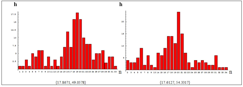
[image:11.595.70.539.440.609.2]

As a result, we obtain histograms that can be compared with the histogram in FigA.3.2-3.

[image:12.595.69.538.138.312.2]

In brackets it is point out values of the estimates

{

m D

_x

,

_x

}

for this realization. Obviously, they well agree with Shnoll experiment (FigA3.2-3), although the statistical fluctuations for the number of samples

M

=

173

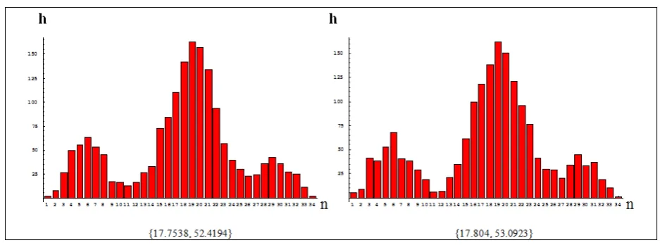
are large enough, and for clarification it is necessary to increase this value by next decimal order. Then the spread will decrease noticeably. We have for the number of samples M=1730the histogram of the form:

Figure A3.6-7. Histograms for some realizations of the mixture of three binomial distributions (number of samples M=1730).

From this we see that if for the realizations Fig.A3.2-3 (Fig.A3.4-5), from statistical fluctuations the error in the determination of peak values are possible, then for the realizations of FigA3.6-7 number of samples is already sufficient large, and these peak values can be determined practically accurately.

On the basis of this, it can be concluded that in the case of the Shnoll experiment (FigA3.2-3), the mixture can consist of more than three numbers of distributions. However, having only one histogram of the experiment

M

=

173

, and based on the research [12, p. 17-18], we can to make only preliminary conclusions.

1) The stochastic properties of the chemical reaction can be characterized by mixture of binomial distributions.

2) This, most likely, means that the chemical system has several discrete distinguishable states, with different rates of reaction.

3) Causes of transition from the main, most probable state of the chemical system to other, less likely states, can be as internal fluctuations or oscillations, so external influences, as well as their combination.

At the molecular level, this may mean that there are several discrete states of the protein molecule or other substance, with different threshold values

E

₀. According to the theory set out in Section 6.1 of the Appendix, different

0

E

lead to different values of the rate of chemical reaction. Is this due to the quantum-mechanical properties of the chemical system, or perhaps it is possible classic description, judging by the state of the research, now as yet is difficulty to determine.

In any case, in this Shnoll experiment is actually found an interesting effect of the discrete rates of the chemical reaction, leading to significant deviations from a priori theoretical expectations. As reasonably noted in [12], there is

need for further complicated and laborious studies.

6.4. Histograms Shape Similarity

At analyzing the Shnoll effect, researchers use a qualitative concept – «Histograms Shape Similarity» (HSS). A quantitative description of this concept is not presented, nor is it given a physical definition of this.

In practice, one of the methods to determine the HSS consist in some smoothing out the shape of the histograms, laying over their graphs on each other for expertly subjective estimate – is there similarity or not. This corresponds to the most primitive method of estimation «by eye» by principle «fit-unfit» for the quality of «wares» on the works, using the simplest two-level scale. However, to deny the possibility of such a method for the problem of «proving the existence of the Shnoll effect», as some of his opponents do, is not constructive.

We will seek a strict definition of the concept of HSS in order to obtain a wider scale of estimation and to exclusion the subjective factor of it.

Obviously, the concept of HSS in the general case should be applicable to any uniformity histograms. In the simplest case, these are histograms of a random process with two different states (such as tossing a coin), consisting of two rectangles with a unity base.

Such histograms will be called bi-component.

Suppose that series of experiments are carried out and their results are presented in the form

{

} {

}

}

{

h x1, 1 , ,h x2 2 _i, h1,i+h2,i =Ni, where

N

i – number

of all tests in

i th

−

series.

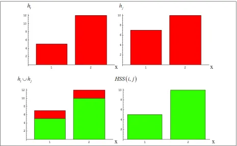
[image:13.595.72.538.87.374.2]

Figure A4.1. Determination of HSS for bi-component histograms

Obviously, as this estimate we can choose the area of the rectangles common to both histograms. For the case

i j

N

=

N

=

N

mathematically this is expressed as

( )

,

( , )

1,i 1,j

( ,

2,i 2,j

)

HSS i j

=

Min h h

+

Min h h

It is not difficult to see that, depending on the different shapes of such histograms, the domain of estimation can take on values

0

≤

HSS N

≤

, i.e. from complete coincidence to complete incompatibility. Thus, in this particular case of the simplest histograms we already have a discrete scale for estimating the HSS in a wide range.

To compare histograms in the case

N

_i

≠

N

_j, then should go to the frequencies of events, which is equivalent to presenting the results in the form

{ } { }

}

{

1

,

1

,

2

,

2 _i

,

i i

,

1,i 2,i

1

i

h

h x

h x

h

h

h

N

=

+

=











_,

and, accordingly, we have a scale of estimates similar to probability, i.e.

0

≤

HSS



≤

1,

where



_{( )}

_,

_{( ,}

_{1,i 1,j}

₎

_{( ,}

_{2,i 2,j}

₎

HSS i j

=

Min h h

 

+

Min h h

 

It is easy to generalize these results for multi-components histograms consisting of rectangles with a unity base, which have representing

{

} {

}

{

}

}

{

1 1 2 2 ,

1

,

,

,

, ... ,

K

,

K _i

,

K k i i

,

k

h x

h x

h x

h

N

=

=

∑

Accordingly, for comparing histograms in the case

N

_i

=

N

_j

=

N

we have

( )

, ,

1

,

K

( ,

k i k j

)

k

HSS i j

Min h h

=

For comparing histograms in the case

N

_i

≠

N

_j, it is necessary get to frequencies, i.e. normalized histograms. We denote

, , k i

k i i

h

h

N

=



_{, and then we obtain generalization of the preceding formulas}

{ } { } {

}

}

{

_{1 1 2 2 ,} 

_{( )}

_{, ,}

1 1

, , , , ... , K, K _i, K k i 1, , K ( ,k i k j)

k k

h x h x h x h HSS i j Min h h

= =

= =

∑

∑

     

The last formulas correspond with histograms – analogues density function (DF) of probability, which does not have infinite jumps. Consequently, the concept of HSS can be generalized to the theoretical DF of random variables

x

having properties

( ) 0,

( )

1

f x

∞

f x dx

−∞

≥

∫

=

Further it will consider DF with finite boundaries, and write the last equation without specifying limits of integration. HSS for two different DF is their joint area, i.e. the projection of one flat figure of a unit area onto another with the same properties



_{( ( ), ( ))}

_{1 2}

_{( , )}

_{1 2}

_{( ( ), ( ))}

_{1 2}

HSS f x f x

= Ρ

f f

=

∫

Min f x f x dx

The last integral has presentation

1 2 1 2

1 2 1 2 1 2

( ) ( ) ( ) ( )

( ( ), ( )) ( ) ( ) 1 ( ) ,

f x f x f x f x

Min f x f x dx f x dx f x dx f f dx+

< >

= + = − −

∫

∫

∫

∫

where it is designation

,

0

0,

0

y y

y

y

+

>



= 

_≤



, and accounted 1 2 1 2

1 1

( ) ( ) ( ) ( )

( )

( )

1

f x f x f x f x

f x dx

f x dx

< >

+

=

∫

∫

.

That presentation transform with account of identity

1 2 1 2 1 2 2 1 1 2

( , )

f f

f x

( )

f x dx

( )

(

f

f dx

)

+

(

f

f dx

)

+

2 (

f

f dx

)

+

Φ

=

∫

−

=

∫

−

+

∫

−

=

∫

−

,

where it is used that

1( ) 2( ) ( 1 2) ( 2 1) 0

f x dx− f x dx= f − f dx+ − f − f dx+ =

∫

∫

∫

∫

.

In result it is presentation 1 2

1 2 1 2

( , ) 1

f f

( , )

f f

Ρ

= − Φ

.

This can be interpreted as the existence of two ways of estimating HSS. If above it was used the method based on estimating the coincident area of the histograms or DF, then it is possible another method, connected with estimation difference of areas of these figures. At the same time, we find that Snoll qualitative approach to the definition of HSS makes sense. They practically visually estimate the proximity of the curves enveloping the histogram and DF, and this estimate corresponds exactly to

Φ

( , )

f f

_{1 2}

=

∫

f x

₁

( )

−

f x dx

₂

( )

– the integrated difference between the two curves.

Although from mathematics point of view both methods are equivalent, but intuition and the empirical approach did not let down the experimenters. A visual qualitative estimate is really more expedient and more accurate to produce with the help

1 2

( , )

f f

Φ

, i.e. difference area, since in formula 1 2

1 2 1 2

( , ) 1

f f

( , )

f f

Ρ

= − Φ

it comes with a multiplier1

2. This already

makes it possible to conclude that the results obtained in Shnoll experiments, despite the qualitative subjective methods of processing experimental data, are quite significant for «proving the existence theorem».

It remains only to remove the existing shortcomings by applying a computer way of processing the measurement results on the basis of the above theory and formulas. Then let's show on a concrete example how to do it.

As the request to provide real experimental data, E.S. Shnoll did not send it, and then we use the resources of the computer program Mathematica with the built-in random number generator (RNG).

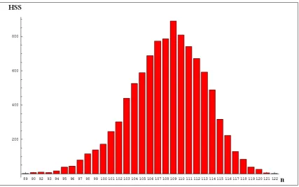
With the help of the RNG is formed the array of primary «experimental data». A random variable is generated by a binomial distribution

Binomial Distribution [n, p] = B [35,18 35]

The mathematical representation of the series has the form

list = {17, 23, 17, 19, 10, ..., 20, 22, 20}.

With the help of subroutine Frequencies [list], this representation is converted to the data for plotting the histogram:

Frequencies [list] = {{3, 10}, {2, 11}, {4, 12}, …, {2, 24},

{2, 26}}.

At

N

=

173

histograms have a graphical representation at the Fig. A4.2.

However now it is not the need to build many such graphs and visually compare them all pair-wise. The entire data array is eventually presented as a matrix with elements

, ,

( ,

),

1...

i k i k i

H h x

i

=

M

. Further all HSS estimates can be calculated automatically. For

M

=

100

and all histograms of this array, we get estimates

HSS H H i j

( ,

_{i j}

),

≠

and in turn get the distribution of these estimates at Fig.A4.4.

For its construction are made

M M

(

−

1) / 2 4950

=

[image:15.595.75.539.220.379.2]

pair-wise comparisons.

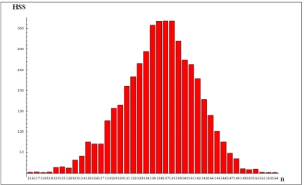
Figure A4.2-3. Histograms for binomial distribution B[35,18₃₅](left) and mixture of three binomial distributions.

[image:15.595.89.521.408.669.2]

At that stage of calculations it is convenient pass to estimate HSS in percentages. For that it is sufficient transform the marks of horizontal scale at formulas

% (

/ ) 100%

HSS

=

HSS N

⋅

For that histogram it is found the diapason of values

% (122 /173 162 /173) 100% (73,5 93,6)%.

HSS

=



⋅

=



For corresponding with some threshold qualitative estimate, we can to set the value of the HSS, down which the histograms are not considered similar. Choosing, as example,

% 90%,

156

HSS

=

HSS

=

, we get that the share of estimate

HSS

% 90%

≥

is relatively small. The choice of this or any another threshold value, in general case cannot have a logical and objective basis and is always conditional. But for estimation tasks of different histograms arrays the threshold value can be chosen, that allows objectively comparing histograms with certain properties. For considered example (Fig.A4.4) the choice of the threshold value

HSS

% 70%

=

corresponds to the fact that for the given experiment all the histograms must be within similarity.

But this may be a consequence of that the distribution of r.v. is enough compact, or the RNG creates a limited «variety» of histograms. In such cases, it is necessary to

analyze the full information about HSS, i.e. of distribution Fig.A4.4. Visual analysis reveals that the form of distribution is well-shaped, without explicit expressed components, and we can conclude in favor of the first assumption, and with respect to RNG this indicates its qualitative functioning.

Consider an array of histograms with a more complex distribution, when r.v. – a mixture of three binomial

distributions:

19 6 29

2 1 2

3

B

[35, ]

35

+

5

B

[35, ]

35

+

15

B

[35, ],

35

N

=

173.

A typical histogram of the «series»

, ,

( ,

),

1...

i k i k i

H h x

′

i

=

M

is shown at Fig.A4.3.

At Fig.A4.5 it is the distribution

HSS H H i j

( ,

i

′ ′

j

),

≠

for comparing «series» by

M

=

100.

% (116 /173 154 /173) 100% (67,0 89,0)%.

HSS

=

_

⋅

=

_

We can see as the spread of values for this r.v. diminished, like the similarity of histograms in general. As if threshold 90% is not achieved at all, but choice of calibration threshold also

% 70%

[image:16.595.90.523.383.646.2]

HSS

=

is valid. It can be concluded that less compact r.v. give less similarity for histograms with all other equal conditions. This computer method is very sensitive to changes in the properties of r.v.