Geomorphometry in Landscape Ecology: Issues of Scale,
Physiography, and Application
Kirsten Erin Ironside
1,*, David J. Mattson1,Terence Arundel
1, Tad Theimer2, Brandon Holton3,Michael Peters4,
Thomas C. Edwards, Jr.
5, Jered Hansen
11U.S. Geological Survey, Southwest Biological Science Center, United States 2Biological Sciences Department, Northern Arizona University, United States
3National Park Service, Grand Canyon National Park, Science and Resource Center, United States 4Pterylae Systems, Arizona, United States
5U.S. Geological Survey, Utah Cooperative Fish and Wildlife Research Unit, Department of Wildland Resources,
Utah State University, United States
Copyright©2018 by authors, all rights reserved. Authors agree that this article remains permanently open access under the terms of the Creative Commons Attribution License 4.0 International License
Abstract
Topographic measures are frequently used ina variety of landscape ecology applications, in their simplest form as elevation, slope, and aspect, but increasingly more complex measures are being employed. We explore terrain metric similarity with changes in scale, both grain and extent, and examine how selecting the best measures is sensitive to changes in application. There are three types of topographic measures: 1) those that relate to orientation for approximating solar input, 2) those that capture variability in terrain configuration, and 3) those that provide metrics about landform features. Many biodiversity hotspots and predators have been found to coincide with areas of complexity, yet most complexity measures cannot differentiate between terrain steepness and uneven and broken terrain. Currently characterizing terrain in landscape-level analyses can be challenging, especially at coarser spatial resolutions but developing methods that improve landscape-level assessments include multivariate approaches and the use of neighborhood statistics. Some measures are sensitive to the spatial grain of calculation, the physiography of the landscape, and the scale of application. We show which measures have the potential to be multi-collinear, and illustrate with a case study how the selection of the best measures can change depending on the question at hand using mountain lion (Puma concolor) occurrence data. The case study showed a combination of infrequently employed metrics, such as view-shed analysis and focal statistics, outperform more commonly employed singular metrics. The use of focal statistics as a measure of topographic complexity shows promise for improving how mountain lions use terrain features.
Keywords
Habitat, Topography, Terrain,Ruggedness, Mountain Lion, Puma concolor
1. Introduction
morphological features for animal locomotion, where species such as the modern day African cheetah (Acinonyx jubatus) has evolved cursorial locomotion and predation, and is able to run for long distances over flat terrain to obtain prey. Whereas a common ancestor, the American puma (Puma concolor) [4], also commonly referred to as mountain lions, is unable to run long distances, and relies on saltatorial (leaping and pouncing) or scansorial (climbing) locomotion for evasion and hunting [5, 6].
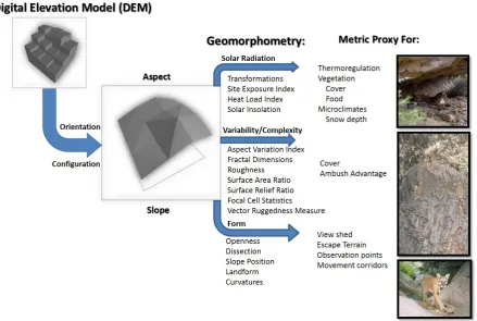
Because terrain has played a significant role in species’ morphological adaptation and evolution, some metric of it is inevitably incorporated into evaluations of species’ habitat requirements. Landscape ecologists conducting analyses related to distribution modeling, wildlife resource selection functions, habitat connectivity, or simulating movement patterns, frequently incorporate topographic features to describe how organisms or genes are distributed across environments. Many of these metrics serve as an indirect measure of how organisms respond to their environment (Figure 1). For example, aspect may serve as a proxy for evapotranspiration rates that are directly related to vegetation growth, distribution, and structure [7]. In turn, the vegetation associated with particular aspects may be selected by various animal species for food and cover. Terrain configurations that result in a large degree of heterogeneity of aspects and form have in turn been good metrics of species richness [8].
How topographic features are characterized can have pronounced influence on the results of such analyses. The use of GIS in ecology is widespread for understanding the spatial structure of environmental systems from biotic to the abiotic features that influence their occurrence, abundance, and community structure. In practice, landscape ecologists are faced with many options when incorporating topography into analyses of spatial patterns. Options include selecting a metric or metrics to employ, deciding the appropriate spatial grain to calculate them, and, for many topographic metrics, choosing an appropriate analysis window. Analysis windows can be set in various shapes (circular, rectangular, oblong, etc.) and be conceptually infinite in size. The similarity of one terrain metric to another is not always clear, nor the degree of sensitivity to changes in specification and application. When comparing one study to another employing a different metric, the influence of using a different topographic measure on results is not easily ascertained for most. Little consensus exists on which measures are the most appropriate for various applications.
Geomorphometric measures are predominately of two types, those concerned with orientation of topographic
features and those concerned with landscape configuration - the most commonly derived metrics being aspect and slope (Figure 1). Efforts to improve how the orientation of topographic features relates to solar input have resulted in numerous metrics for quantifying solar radiation, from simple mathematical transformations of aspect to complex models of solar insolation that account for seasonal changes in sunlight, latitude, and shadowing [9-11]. Efforts to capture the heterogeneity of three-dimensional characteristics of land or benthic surfaces have been described as those capturing topographic complexity, and are commonly referred to as roughness or ruggedness measures. Many metrics were developed to measure the form of topographic features for geomorphology and landform classification schemes (Figure 1). Various metrics fall into this category such as those used for measuring exposure, view-sheds, topographic positioning, and curvatures of features. Often these continuous variables are classified into various landform descriptions such as valleys, toe-slopes, ridges, draws, peaks, etc. [12] and have a strong association with soil and hydrological characteristics [1]. Similar to the effect of aspect, landforms have been associated with plant growth and structure [13, 14] and how animals move through the landscape [15].
Figure 1. Digital Elevation Models (DEMS) are used for a variety of landscape metrics, sometimes just as raw 3-dimensional coordinates, and often as slope and aspect. Several other metrics have been developed for quantifying the effects of solar radiation, including several transformations of aspect, indices of relative solar inputs, and complex models of solar insolation. Measures of orientation have strong influences on vegetation, evapotranspiration, and snow accumulation. DEMs have also been used to quantify topographic complexity and landforms. These metrics can serve as proxies, such as slope, which is often used to describe escape terrain for bighorn sheep, and mountain lions have been described as selecting for rugged terrain. Photographs courtesy of the U.S. Geological Survey.
Geomorphometry adds another level of complexity related to scale that remains largely unexplored. For many metrics an analysis window must be set, resulting in an extent within an extent, which can be specified for various shapes, sizes, and directionality. We did not explore the effects of variation in the size and shape of the analysis window and this is an area in need of further research. For most reviewed metrics that we calculated to explore the effects of scale (grain and study area extent), the default rectangular 3x3 cell analysis window was used. Issues related to how parametrization of analysis windows are specified have been explored by Wood [22] and methods are available in Landserf software for exploring sensitivities of the analysis window to scale (www.landserf.org). Future planned versions of the FRAGSTATS software program will also incorporate neighborhood statistics of continuous variables, in addition to the landscape-level spatial patterns of categorical mapping already implemented
(http://www.umass.edu/landeco/research/fragstats/fragstat s.html).
Most evaluations of the relationship between biotic factors and topography are equivalent to quantifying the association with or distance from particular topographic
features, without consideration of the surrounding conditions. We explore the use of focal cell statistics (e.g. neighborhoods) to describe terrain variability of a given area, capturing the degree of undulation, and explore the idea that animals may be selecting for areas of particular topographic configuration, rather than particular topographic features such as a ridgeline. This is similar to exploring how future planned versions of FRAGSTATS may contribute to improving landscape level analyses.
of community dynamics and richness, shaping species activity patterns, and contributing to evolutionary histories in both marine and terrestrial environments [8, 23-28]. Not only does topography represent a relatively static physical feature of the landscape but it also shapes many indirect and dynamic features of the landscape. For example, orientation has been a good indicator of evapotranspiration rates, snow accumulation and melt-off rates, affecting the timing of green-up, and therefore shaping how many wildlife species use the environment [23]. A previous review found many metrics are very similar to one another, yet calculated differently [23]. We expand on this previous research to explore how changes in grain and study area extent that result in different physical forms being represented, influence similarity between metrics. The physiography of areas covered includes a large canyon system, a volcanic field, a series of mountainous peaks, and a mesa.
2. Materials and Methods
In addition to slope, we evaluate seven measures related to aspect/orientation calculations, eight measures related to capturing topographic complexity and variability, and nine measures that were developed for landform classification. Though many of these measures have traditionally been binned into classification schemes, notably aspect, we prefer a continuous representation of parameters. Cushman et al. [29] argue for landscape ecologists to accurately identify pattern and process across landscapes, so there is a need to adopt a gradient approach and move away from the more traditional patch and mosaic approach to viewing the landscape. We support this view and therefore compare all measures as continuous parameters. Differences in classification schemes add one more level of complexity when attempting to compare studies using different metrics.
We selected metrics that have been implemented in a wide array of landscape and seascape level studies and those geomorphometrics that are readily available in software packages. Most habitat assessments just simply use elevation or depth in marine environments, which can lack theoretical or practical contexts in how organisms are relating to topography. Elevation in this raw form is no more than a referenced position in three-dimensional space, similar to latitude and longitude and can be a misleading topographic measure [23]. For studies that have sought to measure topographic features, there is often reliance on a particular metric by a researcher. The fact that no metric has gained wide acceptance among researchers (other than the uninformative use of elevation), suggests terrain may need several combinations of metrics to adequately describe the landscape [23, 28]. The few explorations into multivariate characterization of
topography in investigations of wildlife resource use, suggest this approach is optimal [2, 23, 30, 31].
In support of this multivariate approach, we provide similarity metrics between measures, by providing correlation coefficients which are commonly used to screen variables for potential problems with multicollinearity [32], or as criteria to combine into principle components. We also cover a wide range of physiographic features and change in scale to demonstrate their effects on metrics. Lastly, we explore ways to implement the use of geomorphometrics in resource selection of a large mobile predator, often associated with areas of topographic complexity in the western North American portion of its range.
We used two GIS software packages, ArcGIS v10.2 [33] and LandSerf [22]. Additionally, we used Python 2.7 scripts in ArcGIS or as stand-alone processes. ArcGIS calculations included the use of the Spatial Analyst extension and custom GIS python scripts developed by Evans et al. [34] and the authors here [35]. Measures were calculated from 1 x 1-degree DEM tiles obtained from the 1 arc second USGS seamless National Elevation Dataset (NED) [29]. Processing steps included mosaicking tiles for the study area extent, projecting from the native geographic coordinate system to Universal Transvers Mercator (UTM) North American Datum of 1983 (NAD83) zone 12 north, and running focal statistics using a 2-cell circular radius bilinear resampling window to remove artifacts or pits in the DEM [12]. The cell size was set to 30-m resolution. We created a second DEM dataset from this 30-m dataset, by resampling using bilinear resampling to a 1-km resolution.
2.1. Orientation
Measures numbered one through six were calculated using the Geomorphometric and Gradient Metrics Toolbox [34] in ArcGIS v10.2 [33].
2.1.1. Linear Aspect
It transforms circular aspect, in radians, to a linear variable using focal statistics for a given window. Focal statistics for a given window (defaults to 3x3) is run for:
𝐴𝐴𝐴𝐴𝐴𝐴𝐴𝐴𝐴𝐴𝐴𝐴𝑠𝑠= sin(180𝜋𝜋 �2𝜋𝜋 +𝜋𝜋2� − 𝐴𝐴𝐴𝐴𝐴𝐴𝐴𝐴𝐴𝐴𝐴𝐴𝑟𝑟𝑟𝑟𝑟𝑟𝑟𝑟𝑟𝑟𝑟𝑟𝑠𝑠)/180𝜋𝜋 (1)
𝐴𝐴𝐴𝐴𝐴𝐴𝐴𝐴𝐴𝐴𝐴𝐴𝑐𝑐= cos(180𝜋𝜋 �2𝜋𝜋 +𝜋𝜋2� − 𝐴𝐴𝐴𝐴𝐴𝐴𝐴𝐴𝐴𝐴𝐴𝐴𝑟𝑟𝑟𝑟𝑟𝑟𝑟𝑟𝑟𝑟𝑟𝑟𝑠𝑠)/180𝜋𝜋 (2)
(3) 2.1.2. COS and SIN Transformations of Aspect
These metrics assume the northeast azimuth of 45° is a maximum and the southwest quadrant can be an empirically derived minimum [7]. For slopes from 0% - 100%, the functions are linearized and bounded from -1 to 1 and slopes greater than 100% are treated as no data.
𝐴𝐴𝐴𝐴𝐴𝐴𝐴𝐴𝐴𝐴𝐴𝐴𝑙𝑙𝑙𝑙𝑙𝑙𝐴𝐴𝑙𝑙𝑙𝑙 = �180𝜋𝜋 �2𝜋𝜋 +𝜋𝜋2� − arctan �𝐴𝐴𝐴𝐴𝐴𝐴𝐴𝐴𝐴𝐴𝐴𝐴𝐴𝐴𝐴𝐴𝐴𝐴𝐴𝐴𝐴𝐴𝐴𝐴𝐴𝐴 𝐴𝐴�
180 𝜋𝜋 � 𝑚𝑚𝑚𝑚𝑚𝑚 2𝜋𝜋(
2.1.3. Topographic Radiation Aspect Index (Transformed Aspect - TRASP)
Circular aspect is transformed to a value of zero for north- northeast azimuths, and a value of one for southwesterly azimuths, resulting in a continuous variable between 0 – 1 [36];
TRASP = 1 –cos (�180π��Aspect°-30�)
2 (4)
2.1.4. Site Exposure Index (SEI)
Circular aspect is rescaled to a north/south axis and is weighted by the steepness of the slope on a scale from -100 to 100 [37];
SEI = θ́cos (πα-180180 ) (5) 2.1.5. Heat Load Index (HLI)
Southwest facing slopes are found to be warmer than a southeast facing slope, even though the amount of solar radiation they receive is equivalent. HLI accounts for this by "folding" the aspect so that the highest values are southwest and the lowest values are northeast. In addition, this method includes steepness of slope. This index ranges from 0 (coolest) to 1 (hottest) [38];
𝑓𝑓𝑠𝑠= |π − |𝑆𝑆𝑙𝑙𝑚𝑚𝐴𝐴𝐴𝐴𝑟𝑟𝑟𝑟𝑟𝑟𝑟𝑟𝑟𝑟𝑟𝑟𝑠𝑠−5π4 || (6)
HLI 0.039 [0.808*cos (l)*cos
(θ)]--[0.196*sin (θ)]-[0.482*cos (fs*sin (fs)) (7)
2.1.6. Solar Insolation
We used ArcGIS v10.2 [33] Spatial Analyst extension to calculate an annual global solar insolation raster. The solar radiation analysis tools calculate insolation across a landscape based on methods from the hemispherical view-shed algorithm initially developed by Rich et al. [10, 11] and further developed by Fu & Rich [39, 40].
2.2. Complexity
2.2.1. Aspect Variation Index (AVI)
We used ArcGIS v10.2 [33] Spatial Analyst extension to calculate a measure of topographic complexity used in Neilson et al. [41] that measures variability in aspects. Aspect variation was measured in a rectangular 3x3 cell analysis window using Spatial Analyst’s Neighborhood focal statistics variation (count of different aspect classes in the surrounding cells) for an aspect raster reclassified into flat, N, NE, E, SE, S, SW, W, and NW (the default classes in Spatial Analysts aspect tool). Average slope was measured in a rectangular 3x3 cell analysis window using Spatial Analyst Neighborhood focal statistic's mean function.
AVI = (aspect variation x average slope)
/(aspect variation + average slope) (8)
2.2.2. Fractal Dimensions (D)
We used Landserf v2.3 [22] to calculate fractal dimensions using the minimum allowable analysis window of 9x9 cells. Fractal dimensions are indices of geometric irregularity of a surface with flat values given a value of 2 and infinitely “crumpled” surfaces having values of 3. Surfaces with values of 2 are often bodies of water or other perfectly level features on the landscape. D is an indicator of relief complexity derived from a fractal Brownian motion model and variograms [42]. The expected value of the squared elevation difference between two DEM cells, p and q, is;
∑(Zp-Zq)2= k�dpq�2H (9)
where the variance is calculated using the mean of the squared height and H equals 3-D
D = 3-(b2) (10) where b is the slope of a log-log plot of variance against distance
2.2.3. Surface Area Ratio (SAR)
We calculated SAR using the Geomorphometric and Gradient Metrics Toolbox [34] in ArcGIS v10.2 [33], a metric developed to capture rugosity, by calculating the ratio of surface area to planar area [43, 44]. Surface area is calculated using triangulated irregular networks (TINs) calculated from DEMs and planar area calculated from the analysis window of the DEM.
2.2.4. Roughness
We calculated roughness using the Geomorphometric and Gradient Metrics Toolbox [34] in ArcGIS v10.2 [33]. This measure is also commonly referred to as the terrain ruggedness index (TRI) Riley [45-47], which is a focal cell statistic of the variance in elevation values for a given analysis window. Here it is calculated as the focal square-root of the summed differences in elevations of neighboring cells for a 3x3 analysis window.
2.2.5. Standard Deviation of Elevation
We included a focal cell statistic as a potential measure of topographic complexity by using ArcGIS v10.2 [33] and the Spatial Analyst extension. The standard deviation, the variance about the mean, of a rectangular analysis window of 3x3 cells was calculated from the DEMs.
2.2.6. Standard Deviation of Total Curvature
2.2.7. Vector Ruggedness Measure (VRM)
We used a VRM Python script written for ArcGIS v10.2 [33] to calculate this measure of ruggedness by Sappington et al. [2]. VRM is a standardized measure of the three-dimensional dispersion of vectors orthogonal to slope gradients and aspects of a surface derived from DEMs.
(11) where n is the number of cells in the neighborhood and the vectors x. y, and z are equal to
z = cos(s); x=xy×sin(α); xy=sin(α);
and y=xy×cos(α) (12) where s is the orthogonal slope and α is the angle between the orthogonal slope and the vectors
2.2.8. Surface Relief Ratio (SRR)
We calculated SRR using the Geomorphometric and Gradient Metrics Toolbox [34] in ArcGIS v10.2 [33]. SSR is a measure of rugosity or ruggedness of a continuous raster surface developed by Pike & Wilson [48]. We used the default rectangular 3x3 cell analysis window.
𝑆𝑆𝑆𝑆𝑆𝑆 = z� (s)−z(s)min
z(s)max−z(s)min (13) where z is the elevation and s is the analysis window size.
2.3. Form
2.3.1. Positive Openness
We calculated positive openness using the methods of Yokoyama et al. [49] in Python 2.7 [35]. Positive openness is an index incorporating the terrain line-of-sight, or view-shed concept for measuring terrain exposure to the sky and is calculated from a DEM by averaging the zenith angles that are within an arbitrary radius from a central cell for each cardinal and ordinal direction. Openness has high values for convex landforms and low values for concave landforms. Positive openness was calculated using a 480-meter search radius.
2.3.2. Dissection
We calculated dissection using the Geomorphometric and Gradient Metrics Toolbox [34] in ArcGIS v10.2 [33]. Dissection is a measure meant to describe a location’s configuration relative to surrounding locations. Evans et al.’s [34] toolbox implements Martonne’s modified dissection [50] which is calculated as:
(14)
where z is the elevation, i is the focal cell, and s the analysis window size.
2.3.3. Slope Position
We calculated slope position using the Geomorphometric and Gradient Metrics Toolbox [34] in ArcGIS v10.2 [33]. Slope position, also known as Topographic Position Index (TPI) is calculated using the methods in De Reu et al. [51] and Guisan et al. [52]. This metric calculates scalable slope position by subtracting the average neighbor values from the focal value. Positive values indicate that the central point is located higher than its average surroundings, while negative values indicate a position lower than the average.
2.3.4. Landform
We calculated landform curvature using the Geomorphometric and Gradient Metrics Toolbox [34] in ArcGIS v10.2 [33]. Measuring curvatures has been a popular geomorphometric for landform classifications as they capture convexity and concavity. Evans et al. [34] use Bolstad’s variant [51] of surface curvature, an index based on features that confine the view from the focal cell of a 3x3 cell window of analysis. A correction measure for edges is used by dividing by the radius to the outermost cell [52, 53].
2.3.5. Curvatures
Many variants of curvature calculations exist. Here we include cross-sectional and longitudinal curvature calculations available in Landserf v 2.3 [22] and the total, profile, and plan curvature calculations [13, 14] available in ArcGIS v10.2 [33] Spatial Analyst extension. Similar to the landform calculation above, these are meant to measure convexity and concavities in various directions using the second derivative.
2.4. Case Study
2.4.1. Effects of Changes in Grain and Physiography on Correlations between Metrics
Our case study explores wildlife resource selection applications where topography plays a strong role in habitat selection and detectability. Many wildlife population surveys can be influenced by terrain, either altering visibility or by making access logistically difficult [54]. Marking animals with GPS or radio tracking devices is a common study method to monitor animal movements over landscapes, but is also known to be biased by terrain that blocks satellite and radio signals [55, 56]. We explore how a landscape level of analysis is conducted can affect which measures are selected by alternating sampling design and correcting for sampling bias.
extent encompasses several different landforms and is also the location of a long-term study of mountain lions, Puma concolor, that were tagged with GPS telemetry collars (Figure 2) [57]. We evaluated how similar metrics are to one another using Pearson product moment correlation, which evaluates the linear relationship between two continuous variables using Minitab 17 statistical software. We compare the entire study area at 1-km resolution and 30-m resolution using a random sample of 72,804 cells within the study area boundaries (Figure 2A). We then subdivide the study area based on selected home-ranges of mountain lions, equivalent to the 90th isopleth of utilization distributions calculated using the Local Convex Hull (LoCoH) method [58], that represent distinct physiographies within the study area (Figure 2). We represent the following landforms: canyons (Figure 2B), gentle rolling hills (Figure 2C), an inactive volcanic field of cinder cones (Figure 2D), mountainous peaks (Figure 2E), and mesa/plateau (Figure 2F). These areas are calculated and compared at a 30-m resolution. Standard deviation and coefficients of variation of the correlation coefficients were calculated across the five sub-regions to measure sensitivity of metric similarity due to changes in extent and physiography.
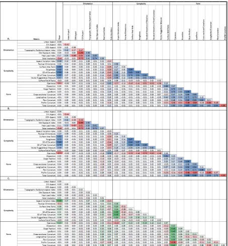
In general, most measures were more related to one another when calculated at a coarser scale (1-km), but not all metrics responded similarly (Figure 3). As a group, measures of orientation were largely not affected in their relationship to one another by the change in grain. The correlations between slope and measures of topographic complexity were stronger at the coarser resolution than the finer resolution. The Aspect Variation Index was the most sensitive to change in scale in its relationship with slope, with it being more correlated at the 1-km resolution. Similarly, it was more similar to the other complexity measures at the coarser scale. Measures of topographic form had the most congruent response as a group, where most measures were slightly more correlated at the 1-km
resolution. Positive openness was found to be the most sensitive to scale change for measures of form. It also is a rather unique measure with relationships to slope, solar insolation, complexity metrics, and form metrics. At a 1-km resolution, it was less inversely related to slope and complexity measures, than at 30-m. At 1-km resolution, openness is more positively related to measures of form than at 30-m (Figure 3).
Figure 2. Study area hillshade (A.) shown with all GPS locations
[image:7.595.308.535.182.476.2]Figure 3. Heat map Pearson correlation coefficient matrix for metrics calculated at 1 km resolution (A.) and 30-m resolution (B.) with shades of blue showing strong positive correlations and shades of red strong negative correlations. The difference in correlation coefficients between scales is shown in part C.
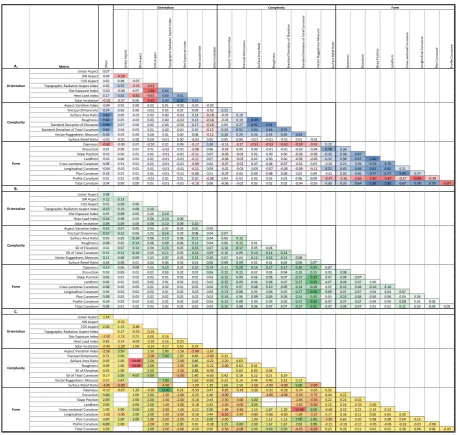
Changes in physiography also influence the similarity between measures within and between groups. The mean correlation across the five different sub-regions is shown in Figure 4A. Using standard deviation of the correlation coefficients across the five physiographic regions as a measure of sensitivity to change, we found Vector Ruggedness Measure to be the most sensitive (Figure 4B), though most metrics varied to some degree with changes in physiography and extent. Using coefficients of variation (Figure 4C) showed variation between groups for cross correlations of orientation and complexity, and complexity
and form. The most variable were sine of aspect, openness, and standard deviation of total curvature. Metrics within groups of orientation and form were relatively stable with the changes in extent. Most metrics that showed sensitivity to changes in physiography had low correlation coefficients, and those with high Pearson correlation coefficients were relativity stable in their similarity with one another across extents.
has been conducted (Northern Arizona University IACUC Protocol # 02-082-R4) in northern Arizona from 2003-2014 by the U.S. Geological Survey and the National Park Service, resulting in the GPS tracking and monitoring of 58 study animals (Figure 2). We evaluate two scales of application, one at a population level and the other at the level of an individual. The population-level analysis includes all observations from all mountain lions monitored in northern Arizona compared to an equal sample of random background conditions across the study area. At the level of an individual we accounted for the movement capacity of the individual using step-lengths. We explore the effects of bias correction on metric selection by weighting observations by the inverse probability of obtaining a GPS fix [35, 56]. Because the probability of obtaining a fix is strongly related to topographic exposure (positive openness) in the model we employ [49], this has the potential to influence which measures are selected in a model selection framework.
For the population-level analysis we compared topographic complexity and form metrics at a weighted 1-km resolution, a weighted 30-m resolution, and an unweighted 30-m resolution. We used changes in deviance to rank measures best describing where mountain lions occur versus an equally sized random background sample of the study area. This represents a coarse resolution analysis in space and time, meant to encompass broad-scale average selection for a multitude of life-stages and activities. We hypothesize that there is an interaction between topography and vegetative cover as a mountain lion moves across the landscape. It is likely they prefer some type of cover at all times, either via the darkness of night when active, or in the form of vegetative cover and/or rough terrain during the day. Therefore, all topographic metrics of terrain had interaction terms with vegetation height in logistic regression models of use versus
availability [62] using the LANDFIRE Existing Vegetation Height (EVH) [63] dataset. We also hypothesized that topographic selection in mountain lions could result in nonlinear relationships. For example, with slope they may prefer mid-range values, avoiding flat areas and extremely steep cliffs. Therefore, we also entered all topographic metrics as quadratic terms, resulting in competing models formulated as topographic metric + topographic metric2 + EVH + topographic metric x EVH.
Figure. 4. Heat map of mean Pearson correlation coefficient matrix for metrics calculated at a 30-m resolution across five physiographic extents (A.), the associated standard deviation around the mean (B.), and the coefficient of variation (C.).
Lin ea r A sp ec t SI N As pe ct CO S A sp ec t To po gr aphi c R adi at io n A spe ct Inde x Si te E xpo sur e I nde x He at Lo ad I nde x So la r I ns ola tio n As pe ct V ar ia tio n I nde x Fr ac tu al D im en sio ns Su rf ac e A re a R at io Ro ug hne ss St an da rd D ev ia tio n o f E le va tio n St anda rd D ev ia tio n o f T ot al C ur va tur e Vec to r R ug ged nes s M ea su re Su rf ac e R el ief R at io O pe nne ss Dis se ct io n Slo pe P os itio n La ndf or m Cr os s-se ct io na l C ur va tu re Lo ng itudi na l C ur va tur e Pl an C ur va tur e Pr of ile C ur va tu re
Linear Aspect 0.07
SIN Aspect 0.00 -0.58
COS Aspect 0.02 0.08 -0.07
Topographic Radiation Aspect Index 0.00 0.37 -0.33 -0.61
Site Exposure Index -0.02 -0.08 0.07 -1.00 0.62
Heat Load Index 0.17 0.42 -0.62 -0.61 0.63 0.61
Solar Insolation -0.18 -0.07 0.06 -0.92 0.60 0.92 0.52
Aspect Variation Index -0.04 0.02 0.00 0.02 0.01 -0.02 -0.01 -0.03
Fractual Dimensions 0.24 0.06 0.00 -0.01 0.02 0.02 0.09 -0.02 0.22
Surface Area Ratio 0.89 0.05 -0.01 0.03 0.00 -0.03 0.14 -0.18 -0.05 0.19
Roughness 0.86 0.05 -0.01 0.03 0.00 -0.03 0.14 -0.18 -0.03 0.19 0.99
Standard Deviation of Elevation 0.98 0.07 0.00 0.02 0.00 -0.02 0.17 -0.18 0.00 0.27 0.92 0.91
Standard Deviation of Total Curvature 0.66 0.04 0.03 0.01 0.00 -0.01 0.10 -0.15 0.24 0.51 0.64 0.66 0.72
Vector Ruggedness Measure 0.34 0.03 0.00 0.00 0.01 0.00 0.08 -0.12 0.30 0.29 0.30 0.35 0.40 0.64
Surface Relief Ratio -0.01 -0.01 0.00 0.00 -0.01 0.00 -0.03 0.05 0.05 0.06 -0.01 -0.01 -0.01 0.01 -0.01
Openness -0.60 -0.09 0.07 -0.10 0.01 0.09 -0.17 0.30 -0.13 -0.27 -0.53 -0.53 -0.61 -0.59 -0.43 0.22
Dissection 0.01 0.00 0.01 0.01 -0.02 -0.01 -0.08 0.06 -0.03 0.00 0.00 -0.01 -0.01 -0.03 -0.04 0.78 0.36
Slope Position 0.03 0.00 0.01 0.01 -0.01 -0.01 -0.11 0.07 -0.06 -0.03 0.02 0.00 0.00 -0.06 -0.06 0.32 0.38 0.67
Landform 0.03 0.00 0.01 0.01 -0.01 -0.01 -0.11 0.07 -0.06 -0.03 0.02 0.00 0.00 -0.06 -0.06 0.32 0.38 0.67 1.00
Cross-sectional Curvature 0.08 0.01 0.01 0.01 -0.01 -0.01 -0.09 0.02 -0.07 -0.02 0.07 0.06 0.07 -0.01 0.03 -0.05 0.23 0.36 0.70 0.70
Longitudinal Curvature -0.04 -0.01 0.01 0.01 -0.01 -0.01 -0.11 0.09 -0.02 -0.03 -0.05 -0.07 -0.06 -0.09 -0.11 0.52 0.40 0.66 0.82 0.82 0.21
Plan Curvature 0.10 0.01 0.01 0.01 -0.01 -0.01 -0.08 0.01 -0.07 0.00 0.09 0.08 0.08 0.02 0.04 -0.01 0.20 0.40 0.77 0.77 0.93 0.27
Profile Curvature 0.01 0.01 0.00 -0.01 0.01 0.01 0.10 -0.08 0.04 0.02 0.02 0.03 0.03 0.06 0.09 -0.47 -0.36 -0.65 -0.87 -0.87 -0.27 -0.96 -0.39
Total Curvature 0.04 0.00 0.00 0.01 -0.01 -0.01 -0.10 0.06 -0.06 -0.02 0.03 0.02 0.02 -0.04 -0.05 0.30 0.35 0.64 0.99 0.99 0.67 0.78 0.79 -0.87
B.
Linear Aspect 0.08
SIN Aspect 0.12 0.13
COS Aspect 0.05 0.09 0.06
Topographic Radiation Aspect Index 0.13 0.10 0.08 0.10
Site Exposure Index 0.05 0.09 0.05 0.00 0.10
Heat Load Index 0.14 0.08 0.03 0.06 0.10 0.06
Solar Insolation 0.08 0.09 0.06 0.09 0.10 0.09 0.10
Aspect Variation Index 0.10 0.07 0.05 0.03 0.02 0.03 0.05 0.05
Fractual Dimensions 0.17 0.12 0.06 0.03 0.14 0.03 0.08 0.04 0.07
Surface Area Ratio 0.05 0.05 0.14 0.06 0.10 0.06 0.12 0.04 0.06 0.12
Roughness 0.08 0.05 0.14 0.06 0.09 0.06 0.12 0.04 0.06 0.12 0.01
SD of Elevation 0.02 0.07 0.12 0.04 0.13 0.05 0.15 0.07 0.10 0.17 0.05 0.04
SD of Total Curvature 0.11 0.12 0.14 0.05 0.11 0.05 0.14 0.09 0.10 0.09 0.14 0.14 0.14
Vector Ruggedness Measure 0.11 0.08 0.09 0.03 0.07 0.03 0.13 0.10 0.07 0.04 0.12 0.14 0.13 0.08
Surface Relief Ratio 0.04 0.06 0.01 0.02 0.04 0.02 0.03 0.06 0.08 0.09 0.02 0.02 0.04 0.06 0.07
Openness 0.13 0.06 0.09 0.03 0.13 0.03 0.10 0.14 0.11 0.20 0.14 0.17 0.17 0.20 0.24 0.07
Dissection 0.03 0.05 0.01 0.02 0.03 0.02 0.02 0.06 0.12 0.11 0.02 0.03 0.04 0.10 0.15 0.03 0.08
Slope Position 0.06 0.01 0.02 0.02 0.01 0.02 0.02 0.03 0.15 0.09 0.06 0.08 0.07 0.17 0.33 0.07 0.09 0.07
Landform 0.06 0.01 0.02 0.02 0.01 0.02 0.02 0.03 0.15 0.09 0.06 0.08 0.07 0.17 0.33 0.07 0.09 0.07 0.00
Cross-sectional Curvature 0.08 0.02 0.03 0.01 0.02 0.01 0.02 0.04 0.13 0.07 0.08 0.10 0.09 0.14 0.18 0.03 0.12 0.08 0.10 0.10
Longitudinal Curvature 0.04 0.02 0.02 0.02 0.01 0.02 0.02 0.04 0.13 0.08 0.04 0.06 0.05 0.17 0.36 0.09 0.07 0.07 0.04 0.04 0.07
Plan Curvature 0.08 0.02 0.03 0.02 0.02 0.02 0.02 0.03 0.14 0.06 0.09 0.09 0.09 0.14 0.20 0.03 0.13 0.08 0.06 0.06 0.04 0.04
Profile Curvature 0.04 0.02 0.02 0.02 0.01 0.02 0.02 0.03 0.13 0.08 0.04 0.05 0.05 0.17 0.35 0.07 0.07 0.07 0.04 0.04 0.09 0.01 0.03
Total Curvature 0.06 0.01 0.02 0.02 0.02 0.02 0.02 0.03 0.15 0.08 0.06 0.07 0.07 0.17 0.31 0.07 0.09 0.07 0.01 0.01 0.11 0.03 0.05 0.03
C.
Linear Aspect 1.14
SIN Aspect -0.22
COS Aspect 2.50 1.13 -0.86
Topographic Radiation Aspect Index 0.27 -0.24 -0.16
Site Exposure Index -2.50 -1.13 0.71 0.00 0.16
Heat Load Index 0.82 0.19 -0.05 -0.10 0.16 0.10
Solar Insolation -0.44 -1.29 1.00 -0.10 0.17 0.10 0.19
Aspect Variation Index -2.50 3.50 1.50 2.00 -1.50 -5.00 -1.67
Fractual Dimensions 0.71 2.00 -3.00 7.00 1.50 0.89 -2.00 0.32
Surface Area Ratio 0.06 1.00 -14.00 2.00 -2.00 0.86 -0.22 -1.20 0.63
Roughness 0.09 1.00 -14.00 2.00 -2.00 0.86 -0.22 -2.00 0.63 0.01
SD of Elevation 0.02 1.00 2.00 -2.50 0.88 -0.39 0.63 0.05 0.04
SD of Total Curvature 0.17 3.00 4.67 5.00 -5.00 1.40 -0.60 0.42 0.18 0.22 0.21 0.19
Vector Ruggedness Measure 0.32 2.67 7.00 1.63 -0.83 0.23 0.14 0.40 0.40 0.33 0.13
Surface Relief Ratio -4.00 -6.00 -4.00 -1.00 1.20 1.60 1.50 -2.00 -2.00 -4.00 6.00 -7.00
Openness -0.22 -0.67 1.29 -0.30 13.00 0.33 -0.59 0.47 -0.85 -0.74 -0.26 -0.32 -0.28 -0.34 -0.56 0.32
Dissection 3.00 1.00 2.00 -1.50 -2.00 -0.25 1.00 -4.00 -3.00 -4.00 -3.33 -3.75 0.04 0.22
Slope Position 2.00 2.00 2.00 -1.00 -2.00 -0.18 0.43 -2.50 -3.00 3.00 -2.83 -5.50 0.22 0.24 0.10
Landform 2.00 2.00 2.00 -1.00 -2.00 -0.18 0.43 -2.50 -3.00 3.00 -2.83 -5.50 0.22 0.24 0.10 0.00
Cross-sectional Curvature 1.00 2.00 3.00 1.00 -2.00 -1.00 -0.22 2.00 -1.86 -3.50 1.14 1.67 1.29 -14.00 6.00 -0.60 0.52 0.22 0.14 0.14
Longitudinal Curvature -1.00 -2.00 2.00 2.00 -1.00 -2.00 -0.18 0.44 -6.50 -2.67 -0.80 -0.86 -0.83 -1.89 -3.27 0.17 0.18 0.11 0.05 0.05 0.33
Plan Curvature 0.80 2.00 3.00 2.00 -2.00 -2.00 -0.25 3.00 -2.00 1.00 1.13 1.13 7.00 5.00 -3.00 0.65 0.20 0.08 0.08 0.04 0.15
Profile Curvature 4.00 2.00 -2.00 1.00 2.00 0.20 -0.38 3.25 4.00 2.00 1.67 1.67 2.83 3.89 -0.15 -0.19 -0.11 -0.05 -0.05 -0.33 -0.01 -0.08
Total Curvature 1.50 2.00 -2.00 -2.00 -0.20 0.50 -2.50 -4.00 2.00 3.50 3.50 -4.25 -6.20 0.23 0.26 0.11 0.01 0.01 0.16 0.04 0.06 -0.03
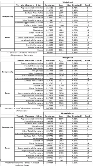
Table 1. Population level resource selection model comparisons
.
Terrain Measure - 1 km Deviance ∆Dev Dev R-sq (adj) Rank
Aspect Variation Index 215526 2680 5.71% 8 Fractual Dimensions 213761 915 6.49% 2 Surface Area Ratio 215152 2306 5.88% 7
Roughness 214891 2045 5.99% 6
SD of Elevation 214279 1433 6.26% 3 SD of Total Curvature 212846 0 6.89% 1
Vector Ruggedness Measure 215977 3131 5.52% 11 Surface Relief Ratio 215952 3106 5.53% 10
Openness 214819 1973 6.02% 5
Dissection 217667 4821 4.78% 18
Slope Position 216505 3659 5.29% 13
Landform 216505 3659 5.29% 14
Cross-sectional Curvature 216925 4079 5.10% 16
Longitudinal Curvature 215814 2968 5.59% 9 Plan Curvature 217238 4392 4.96% 17 Profile Curvature 216126 3280 5.45% 12 Total Curvature 216739 3893 5.18% 15
Slope 214530 1684 6.15% 4
207299 - 9.31%
-Terrain Measure - 30 m Deviance ∆Dev Dev R-sq (adj) Rank
Aspect Variation Index 216602 4886 5.24% 8 Fractal Dimensions 214600 2884 6.12% 3 Surface Area Ratio 215658 3942 5.66% 6
Roughness 215711 3995 5.63% 7
SD of Elevation 215091 3375 5.90% 4 SD of Total Curvature 215555 3839 5.70% 5 Vector Ruggedness Measure 217437 5721 4.88% 14
Surface Relief Ratio 217648 5932 4.79% 18
Openness 211716 0 7.38% 1
Dissection 217456 5740 4.87% 15
Slope Position 217277 5561 4.95% 11
Landform 217277 5561 4.95% 12
Cross-sectional Curvature 217592 5876 4.81% 17 Longitudinal Curvature 217206 5490 4.98% 10 Plan Curvature 217559 5843 4.82% 16 Profile Curvature 217200 5484 4.98% 9
Total Curvature 217279 5563 4.95% 13
Slope 213734 2018 6.50% 2
207854 - 9.07%
-Terrain Measure - 30 m Deviance ∆Dev Dev R-sq (adj) Rank
Aspect Variation Index 192148 1906 4.81% 6
Fractal Dimensions 190242 0 5.75% 1
Surface Area Ratio 193161 2919 4.31% 8
Roughness 193271 3029 4.25% 10
SD of Elevation 191804 1562 4.98% 5 SD of Total Curvature 191743 1501 5.01% 4 Vector Ruggedness Measure 192676 2434 4.55% 7 Surface Relief Ratio 193745 3503 4.02% 16
Openness 191187 945 5.28% 3
Dissection 193224 2982 4.27% 9
Slope Position 193720 3478 4.03% 14
Landform 193720 3478 4.03% 15
Cross-sectional Curvature 193589 3347 4.09% 11 Longitudinal Curvature 193801 3559 3.99% 18 Plan Curvature 193648 3406 4.06% 12 Profile Curvature 193777 3535 4.00% 17 Total Curvature 193716 3474 4.03% 13
Slope 190985 743 5.38% 2
187434 - 7.15%
-Weighted
Complexity
Form Form
Complexity
Form
Weighted
Unweighted
Complexity
SD of Total Curvature + Fractual Dimensions + Openness
Openness + SD of Elevation + Fractual Dimensions
[image:11.595.112.485.92.754.2]3. Results and Discussion
Using competing models to select topographic metrics best explaining where mountain lions occur on the landscape, we found sensitivities to the scale, method of specification, and if detection-bias correction factors were used (Tables 1 and 2). For the population level model (Table 1), including all observations corrected for detection bias, and 1-km resolution metrics, our measure of topographic complexity, standard deviation of total curvature, was ranked number one. Next were fractal dimensions, standard deviation of elevation, and slope. Using the top three ranked variables that are not correlated (defined as < 0.70) resulted in a model including standard deviation of total curvature, fractal dimensions, and openness. Changing the resolution of calculation to a 30-m resolution resulted in openness being the top ranked topographic metric, with slope and fractal dimensions being ranked second and third respectively. Taking the top three ranked uncorrelated metrics resulted in a model using openness, standard deviation of elevation, and fractal dimensions. Staying at the 30-m resolution but not weighting the observations to correct for detection bias, resulted in fractal dimensions being the top-ranked metric. This was followed by slope and openness. A model using the top three uncorrelated metrics resulted in including fractal dimensions, slope and the aspect variation index.
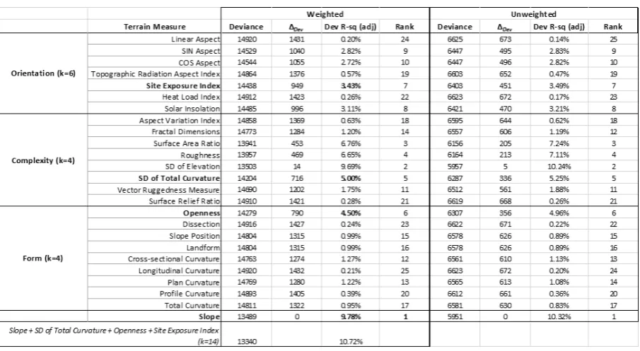
When we subsetted the dataset to observations of a single cougar whose home range encompassed the San Francisco Peaks and Mount Elden (Figure 2E) the top ranked variables changed once again (Table 2). For both the weighted and unweighted model comparisons, slope, standard deviation of elevation, and surface area ratio were
the top-three ranked metrics. Of the orientation measures that were included in these model comparisons, the site exposure index was the top ranked orientation metric. The top four uncorrelated metrics were slope, standard deviation of total curvature, openness, and site exposure index.
We found no one measure had pronounced predictive power over the others and the most deviance was explained by multivariate models incorporating several characteristics of the terrain in our study area. How the models were approached in terms of scale and with the use of correction factors for the effect terrain has on GPS performance, influenced variable selection. How the data were analyzed in terms of a population-wide versus background analysis or that of an individual (accounting for movement capacity) also influenced the best combination of metrics.
[image:12.595.72.525.496.744.2]Because the top ranked variables in our example with mountain lions were often correlated, we chose the next top ranked variable with < 0.70 correlation coefficient to include in the model. This was a driver for the ensemble of metrics to change from comparison to comparison. There was some consistency between the upper-ranked metrics for mountain lions: standard deviation of total curvature, fractal dimensions, openness, slope, and standard deviation of elevation were the most important metrics for measures of complexity and form. The comparison including measures of orientation resulted in the site exposure index (ranked 7th out of 24) being the best metric of orientation. Site exposure index was followed by solar insolation; these two measures of orientation were also highly positively correlated in all of the comparisons.
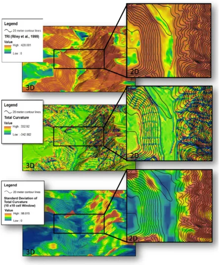
Standard deviation of total curvature was developed during our review to better capture topographic complexity. The typical complexity measures we found do not distinguish between steep slopes and broken or “rugged” terrain [2]. Using focal statistics of the neighborhood around a cell to quantify the variability in form (Figure 5) appears to be a way to identify complex, uneven-faced slopes from flat-faced slopes. At a coarse scale, this appears to best explain the occurrence of mountain lions as a population across our study area. Whether or not the size of area, i.e. the analysis window size, with rugged configuration plays a role in mountain lion resource selection needs further exploration. Characterization of mountain lion use of topography has been addressed by several researchers; Riley [45-47] developed the terrain ruggedness index (TRI) for assessing resource selection of mountain lions in Montana; Dickson et al. [59], Dickson and Beier [15], and Dickson et al. [60] applied the topographic position index (TPI); and Burdett et al. [61] used vector ruggedness measure (VRM) for describing mountain lion movement in southern California. None of these measures ranked high in our model comparisons for northern Arizona, suggesting characterizing topography and how these top predators orient to terrain features on the landscape can be improved upon.
4. Conclusions
Digital elevation models can provide critical information on how organisms relate to terrestrial landscapes. However, the multitude of metrics available and the unknown sensitivities to specification can be overwhelming in applied landscape scale studies. In general, the coarser the spatial grain, the more similar metrics can become, but the degree that terrain measures were affected varied for several metrics. Similarly, changes in extent resulted in some metrics being more sensitive than others in how correlated they were with other metrics, but highly correlated metrics appear to be rather robust to change in physiography. We caution that some measures of topographic complexity are not able to distinguish steepness of slope from uneven or rugged terrain. For mountain lions, we found rarely employed metrics to be the best ranked in model comparisons – first, a metric calculating variation in topographic form, next, another complexity metric, fractal dimensions, and, lastly, one that relies on the view-shed concept of openness. Many wildlife resource selection studies have focused on terrain measures capturing particular features of landscapes such as steepness or a particular landform, but analysis of mountain lions showed configuration of terrain patches and how topography influences visibility to be the most important. How view-sheds are used by animals needs further exploration but could provide meaningful insight into predator-prey dynamics. Metric ranking was
influenced by detection correction measures and is another consideration in relating occurrence with terrain. No single metric outperformed a multivariate approach, suggesting landscape ecologists may not want to rely on a single metric of topography. Quantifying how organisms orient to topography is not resolved and many aspects of how terrain is characterized need further exploration in terms of analysis window affects. The use of focal statistics of continuous measures is an area of landscape quantification that shows promise for improving our understanding of how animals respond to terrain.
Acknowledgements
This study was funded by the NASA Biodiversity and Ecological Forecasting Program (Climate and Biological Response, grant no. NNH10ZFA001N). Financial support for the collection of cougar datasets was provided by the USGS Park-Oriented Biological Support program, the USGS Colorado Plateau Research Station, the NPS Cooperative Conservation Initiative, the Summerlee Foundation, the Wilburforce Foundation, the USGS Southwest Biological Science Center, the USGS Fire Research Program, the Johnson Family Foundation, and Grand Canyon National Park. Material and other in-kind support has been provided by USDA Wildlife Services, The Grand Canyon Trust, Northern Arizona University, Arizona Game and Fish Department, and the NPS Flagstaff Area National Monuments. We thank Kathy Longshore and Dan Thompson for helpful thoughts related to topography and wildlife. We thank Jan Hart, Brian Jansen, Erik York, Sam Dieringer, and JR Murdock for capture, handling, and tagging of mountain lions. We thank Jeffrey Lovich, Amy Whipple and an anonymous reviewer for helpful reviews and comments. The use of trade, product, or firm names in this publication is for descriptive purposes only and does not imply endorsement by the U.S. Government.
REFERENCES
[1] Pike R, Evans I, Hengl T: Geomorphometry: a brief guide. Developments in Soil Science 2009, 33:3-30.
[2] Sappington JM, Longshore KM, Thompson DB:
Quantifying landscape ruggedness for animal habitat analysis: a case study using bighorn sheep in the Mojave Desert. Journal of Wildlife Management 2007, 71:1419-1426.
[3] Tesfa TK, Tarboton DG, Watson DW, Schreuders KA,
Baker ME, Wallace RM: Extraction of hydrological proximity measures from DEMs using parallel processing. Environmental Modelling & Software 2011, 26:1696-1709.
Molecular evolution of mitochondrial 12S RNA and cytochrome b sequences in the pantherine lineage of Felidae. Molecular Biology and Evolution 1995, 12:690-707. [5] Meloro C, Elton S, Louys J, and Bishop LC, Ditchfield P:
Cats in the forest: predicting habitat adaptations from humerus morphometry in extant and fossil Felidae (Carnivora). Paleobiology 2013, 39:323-344.
[6] Bryce CM, Wilmers CC, Williams TM: Energetics and
evasion dynamics of large predators and prey: pumas vs. hounds. PeerJ 2017, 5:e3701.
[7] Stage AR: Notes: An expression for the effect of aspect, slope, and habitat type on tree growth. Forest Science 1976, 22:457-460.
[8] Davies RG, Orme CDL, Storch D, Olson VA, Thomas GH,
Ross SG, Ding T-S, Rasmussen PC, Bennett PM, Owens IP: Topography, energy and the global distribution of bird species richness. Proceedings of the Royal Society of London B: Biological Sciences 2007, 274:1189-1197. [9] Yard MD, Bennett GE, Mietz SN, Coggins LG, Stevens LE,
Hueftle S, Blinn DW: Influence of topographic complexity on solar insolation estimates for the Colorado River, Grand Canyon, AZ. Ecological Modelling 2005, 183:157-172. [10] Rich P, Dubayah R, Hetrick W, Saving S: Using viewshed
models to calculate intercepted solar radiation: applications in ecology. American Society for Photogrammetry and Remote Sensing Technical Papers. In American Society of Photogrammetry and Remote Sensing. 1994: 524-529.
[11] Rich PM, Fu P: Topoclimatic habitat models. In
Proceedings of the fourth international conference on integrating GIS and environmental modeling. 2000: 2-8.
[12] MacMillan R, Shary P, Hengl T, and Reuter H:
Geomorphometry: concepts, software, applications. Elsevier Science. Chap. Landforms and Landforms elements in geomorphometry; 2008.
[13] McNab WH: Terrain shape index: quantifying effect of minor landforms on tree height. Forest Science 1989, 35:91-104.
[14] McNab WH: A topographic index to quantify the effect of mesoscale landform on site productivity. Canadian Journal of Forest Research 1993, 23:1100-1107.
[15] Dickson BG, Beier P: Quantifying the influence of
topographic position on cougar (Puma concolor) movement in southern California, USA. Journal of Zoology 2007, 271:270-277.
[16] Wiens: JA. Spatial scaling in ecology. Functional Ecology 1989, 3:385-397.
[17] Wu J: Effects of changing scale on landscape pattern analysis: scaling relations. Landscape Ecology 2004, 19:125-138.
[18] Wu J, Shen W, Sun W, Tueller PT: Empirical patterns of the effects of changing scale on landscape metrics. Landscape Ecology 2002, 17:761-782.
[19] Urban DL: Modeling ecological processes across scales. Ecology 2005, 86:1996-2006.
[20] Frazier AE: Surface metrics: scaling relationships and
downscaling behavior. Landscape Ecology 2016, 31:351-363.
[21] Frazier AE, Kedron P: Landscape Metrics: Past Progress and Future Directions. Current Landscape Ecology Reports 2017, 2:63-72.
[22] Wood J: Geomorphometry in LandSerf. Developments in Soil Science 2009, 33:333-349.
[23] Bouchet PJ, Meeuwig JJ, Kent S, Chandra P, Letessier TB, Jenner CK: Topographic determinants of mobile vertebrate predator hotspots: current knowledge and future directions. Biological Reviews 2015, 90:699-728.
[24] Kerr JT, Packer L: Habitat heterogeneity as a determinant of mammal species richness in high-energy regions. Nature 1997, 385:252.
[25] Jetz W, Rahbek C: Geographic range size and determinants of avian species richness. Science 2002, 297:1548-1551. [26] Worm B, Lotze HK, Myers RA: Predator diversity hotspots
in the blue ocean. Proceedings of the National Academy of Sciences 2003, 100:9884-9888.
[27] Morato T, Hoyle SD, Allain V, Nicol SJ: Seamounts are hotspots of pelagic biodiversity in the open ocean. Proceedings of the National Academy of Sciences 2010, 107:9707-9711.
[28] Alexander SM: Snow tracking and GIS: using multiple species environment models to determine optimal wildlife crossing sites and evaluate highway mitigation plans on the Trans-Canada Highway. The Canadian Geographer/Le Géographe Canadien 2008, 52:169-187.
[29] U.S. Geological Survey: National Elevation Dataset
(NED)--Raster digital data. (U.S. Geological Survey ed., 2nd edition edition. Sioux Falls: The National Map; 2009. [30] Pittman SJ, Costa BM, Battista TA: Using lidar bathymetry
and boosted regression trees to predict the diversity and abundance of fish and corals. Journal of Coastal Research 2009:27-38.
[31] Larkin D, Vivian-Smith G, Zedler JB: Topographic
heterogeneity theory and ecological restoration. Foundations of restoration ecology 2006:142-164.
[32] Ott RL, Longnecker MT: An introduction to statistical methods and data analysis. Nelson Education; 2015.
[33] Esri: ArcGIS Desktop Release 10.2. Redlands:
Environmental Systems Resource Institute, http://www.esri.com/; 2013.
[34] Evans J, Oakleaf J, Cushman S, Theobald D: An ArcGIS toolbox for surface gradient and geomorphometric modeling, version 2.0-0. Laramie, WY, http://evansmurphywix.com/evansspatial; 2014.
[35] Ironside KE, Mattson DJ, Choate D, Stoner D, Arundel TR, Theimer TC, Holton B, Jansen B, Sexton J, Longshore KM, et al: Variable Terrestrial GPS Telemetry Detection Rates: Parts 1 - 7. (U.S. Geological Survey ed. Flagstaff: U.S. Geological Survey, 10.5066/F7PG1PT2; 2015.
[36] Roberts DW, Cooper SV: Concepts and techniques of
Research Station (USA) 1989.
[37] Balice RG, Miller JD, Oswald BP, Edminster C, Yool SR: Forest Surveys and Wildlife Assessment in the Los Alamos Region: 1998-1999. Los Alamos National Laboratory; 2000.
[38] McCune B, Keon D, Marrs R: Equations for potential
annual direct incident radiation and heat load. Journal of vegetation science 2002, 13:603-606.
[39] Fu P, Rich P: The solar analyst 1.0 user manual. Helios Environmental Modeling Institute 2000, 1616.
[40] Fu P, Rich PM: A geometric solar radiation model with applications in agriculture and forestry. Computers and electronics in agriculture 2002, 37:25-35.
[41] Nielsen SE, Herrero S, Boyce MS, Mace RD, Benn B,
Gibeau ML, and Jevons S: Modelling the spatial distribution of human-caused grizzly bear mortalities in the Central Rockies ecosystem of Canada. Biological Conservation 2004, 120:101-113.
[42] Mark DM, Aronson PB: Scale-dependent fractal
dimensions of topographic surfaces: an empirical investigation, with applications in geomorphology and computer mapping. Mathematical Geology 1984, 16:671-683.
[43] Berry J: Beyond mapping use surface area for realistic calculations. Geo World 2002, 15:20-21.
[44] Jenness JS: Calculating landscape surface area from digital elevation models. Wildlife Society Bulletin 2004, 32:829-839.
[45] Riley SJ: Integration of environmental, biological, and human dimensions for management of mountain lions (Puma concolor) in Montana. Cornell University, 1998. [46] Riley SJ: Index That Quantifies Topographic Heterogeneity.
Intermountain Journal of sciences 1999, 5:23-27.
[47] Riley SJ, Malecki RA: A landscape analysis of cougar distribution and abundance in Montana, USA. Environmental Management 2001, 28:317-323.
[48] Pike RJ, Wilson SE: Elevation-relief ratio, hypsometric integral and geomorphic area-altitude analysis. Geological Society of America Bulletin 1971, 82:1079-1084.
[49] Yokoyama R, Shirasawa M, Pike RJ: Visualizing
topography by openness: a new application of image processing to digital elevation models. Photogrammetric engineering and remote sensing 2002, 68:257-266.
[50] Evans I: General geomorphometry, derivatives of altitude, and descriptive statistics. In Spatial Analysis in Geomorphology. Edited by Chorley RJ. New York: Harper & Row; 1972: 17-90
[51] De Reu J, Bourgeois J, Bats M, Zwertvaegher A, Gelorini V, De Smedt P, Chu W, Antrop M, De Maeyer P, Finke P: Application of the topographic position index to
heterogeneous landscapes. Geomorphology 2013, 186:39-49.
[52] Guisan A, Weiss SB, Weiss AD: GLM versus CCA spatial modeling of plant species distribution. Plant Ecology 1999, 143:107-122.
[53] Bolstad PV, Lillesand T: Improved classification of forest vegetation in northern Wisconsin through a rule-based combination of soils, terrain, and Landsat Thematic Mapper data. Forest Science 1992, 38:5-20.
[54] Bodie WL, Garton EO, Taylor ER, McCoy M: A
sightability model for bighorn sheep in canyon habitats. The Journal of Wildlife Management 1995:832-840.
[55] Frair JL, Fieberg J, Hebblewhite M, Cagnacci F, DeCesare NJ, Pedrotti L: Resolving issues of imprecise and habitat-biased locations in ecological analyses using GPS telemetry data. Philosophical Transactions of the Royal Society of London B: Biological Sciences 2010, 365:2187-2200.
[56] Ironside KE, Mattson DJ, Choate D, Stoner D, Arundel T, Hansen J, Theimer T, Holton B, Jansen B, Sexton JO: Variable terrestrial GPS telemetry detection rates: Addressing the probability of successful acquisitions. Wildlife Society Bulletin 2017.
[57] Mattson DJ: Mountain Lions of the Flagstaff Uplands: 2003-2006 Progress Report. 2007.
[58] Getz WM, Fortmann-Roe S, Cross PC, Lyons AJ, Ryan SJ, Wilmers CC: LoCoH: nonparameteric kernel methods for constructing home ranges and utilization distributions. PloS one 2007, 2:e207.
[59] Dickson BG, Jenness JS, Beier P: Influence of vegetation, topography, and roads on cougar movement in southern California. Journal of Wildlife Management 2005, 69:264-276.
[60] Dickson BG, Roemer GW, McRae BH, Rundall JM:
Models of regional habitat quality and connectivity for pumas (Puma concolor) in the southwestern United States. PloS one 2013, 8:e81898.
[61] Burdett CL, Crooks KR, Theobald DM, Wilson KR,
Boydston EE, Lyren LM, Fisher RN, Vickers TW, Morrison SA, Boyce WM: Interfacing models of wildlife habitat and human development to predict the future distribution of puma habitat. Ecosphere 2010, 1:1-21.
[62] 62. Manly B, McDonald L, Thomas D, McDonald TL,
and Erickson WP: Resource selection by animals: statistical design and analysis for field studies. Springer Science & Business Media; 2007.
[63] LANDFIRE: LANDFIRE 1.1.0--Existing vegetation height and type layers. (LANDFIRE ed., 1.1.0 edition: U.S. Department of Agriculture and U.S. Department of the Interior; 2011.