Abstract - This paper presents the second version of scheduling heuristic to minimize the makespan of a re-entrant flow shop with dominant characteristic at first process. The processes scheduling resembles a four machine permutation re-entrant flow shop with the process routing of M1,M2,M3,M4,M3,M4 in which the first process at M1 has high tendency of exhibiting dominant characteristic. The BAM4 is developed based on the bottleneck correction factor algorithm introduced to the makespan computation using bottleneck approach. It was shown that using bottleneck-based analysis, an effective constructive heuristic can be developed to solve for near-optimal scheduling sequence. At strong machine dominance level and medium to high job numbers, this heuristic shows slightly better makespan performance compared to the NEH. However, for smaller job numbers, NEH is superior.
Keywords – Bottleneck, dominant machine, heuristic, re-entrant flow shop, Scheduling
I. INTRODUCTION
Re-entrant flow shop is one of the important subclass of flow shop which is quite prominent in manufacturing industries. Its special feature is that the job routing may return one or more times to any facility. Among the researchers on re-entrant flow shop, [1] has developed a cyclic scheduling method that takes advantage of the flow character of the re-entrant process where as [2] utilized shortest processing time rule to generate solution with flowtime objective. Concentrating on two machines problem, [3] used dynamic programming approach to achieve makespan objective. The branch and bound technique was utilized by [4,5,6,7] where as the decomposition technique in solving maximum lateness problem for re-entrant flow shop with sequence dependent setup times was suggested by [8]. Mixed integer heuristic algorithms was later on elaborated by [9] in minimizing makespan of a permutation flow shop scheduling problem. Significant works on re-entrant hybrid flow shop can be found in [10,11] where as hybrid algorithms which combine a few well known techniques was reported by [12].
In scheduling literature, there are a number of studies conducted using the bottleneck approach in solving shop scheduling problem. These include shifting bottleneck heuristic [13,14] and bottleneck minimal idleness heuristic [15]. However, not much progress is reported on bottleneck approach in solving re-entrant flow shop problem.
This study contributes into the area of re-entrant flow shop scheduling problem using bottleneck approach. It
explores the capability of the bottleneck approach in developing alternative heuristics to obtain job schedule that generates near optimal makespan. The problem studied in this research can be identified as four machine permutation re-entrant flow shop with the processing route of M1,M2,M3,M4,M3,M4. Several heuristics are being developed to solve this problem and one of them which utilised the absolute bottleneck characteristic was presented in [16]. This paper presents the second version of scheduling heuristic to minimize the makespan of a re-entrant flow shop with dominant characteristic at first process. The heuristic is developed based on the bottleneck correction factor algorithm introduced to the makespan computation using bottleneck approach.
II. BOTTLENECK ADJACENT MATCHING 4 (BAM4) HEURISTIC
The BAM4 heuristic generates a schedule which selects a preceding job based on the best matching index to the last job bottleneck processing time, which is the P1 of the last job (refer Table 1). As a result, minimum discontinuity time between the bottleneck machine of the last job scheduled (P(1,n)) and its subsequent processes is obtained and thus produces near-optimal schedule arrangement. The procedures to implement the BAM4 heuristic to the CMC scheduling are as the followings:
Step 1:
Evaluate the bottleneck dominance level of P(1,j) compared to P(4,j) + P(5,j) + P(6,j) as described in [16]. This is to ensure that P(1,j) is the dominant bottleneck because BAM4 heuristic is more appropriately applicable for this type of bottleneck.
Step 2:
Select the job with the smallest value of P(2,j) + P(3,j) + P(4,j) + P(5,j) + P(6,j) as the last job (nth job). This is in accordance with the makespan formulation under P(1,j) bottleneck characteristics as illustrated in (1) [17].
Makespan =
∑
∑
= =
+
n
j i
n
i
P
j
P
1
6
2
)
,
(
)
,
1
(
+ P1BCF (1) P1BCF = P1 Bottleneck Correction FactorThe formulation above indicated that minimum makespan can possibly be achieved by assigning the job with smallest value of P2+P3+P4+P5+P6 as the last job arrangement.
Step 3:
With the selected last job (nth job) as in Step 2, compute the BAM4 index for the potential n-1 job (second last job) by assuming one by one of the remaining jobs are to be
With Dominant Machine
S. A. Bareduan, S. H. Hasan
assigned as the n-1 job. The BAM4 index is computed as the followings:
For j = n-1,n-2,…,2 BAM4=
∑
∑
∑
∑
= +
= −
= =
− −
+
3
2 1
1 3
2
) 6 , ( )
, 1 ( )
, 4 ( )
, (
i n
j k n
j k i
i P k
P k
VP j
i
P (2)
where j = remaining jobs to be selected one by one VP =Virtual Processing Time as described in [17].
The detail BAM4 index computation is described in the next section.
Step 4:
If available, select the job that has zero BAM4 index. Else, select the job that has the largest negative BAM4 index (negative BAM4 index closest to zero). Else, select the job with the smallest positive BAM4 index. Assign this job for the current job scheduling.
Step 5:
Compute the BAM4 index for job scheduling assignment j = n-2, n-3,…2 one by one using the algorithm at Step 3 and select the best job allocation using Step 4.
Step 6:
Compute the makespan from the completed job scheduling arrangement.
Step 7:
Use the bottleneck scheduling performance 4 (BSP4) index to evaluate the performance of the selected schedule. This index is explained in the next section. If this BSP4 index evaluation suggests that there are other possible last job candidates that may generate better job schedule arrangement, assign these new candidates one by one as the last job and repeat Step 3 to Step 6.
Step 8:
From the entire completed schedule arrangement list, select the schedule that produces the minimum makespan as the best schedule.
III. AN ILLUSTRATIVE EXAMPLE OF BAM4 HEURISTIC
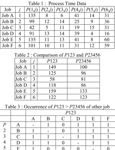
[image:2.595.310.540.71.370.2]Let’s consider the six jobs CMC processes data as in Table 1. First, the P1 bottleneck dominance level is evaluated. This dominance level is measured by detecting the number of occurrences where P1+P2+P3 (or P123) of any job is greater than P2+P3+P4+P5+P6 (or P23456) of other jobs [16]. Table 2 shows the values of P123 and P23456 whereas the occurrences of P123 > P23456 is shown in Table 3. The overall P1 bottleneck dominance level is computed by adding all values in Table 3 which equals to 21. Since this value is more than n(n-1)/2 which is for 6 jobs example problem in Table 1 equals to 6(6-1)/2=15, this means that the bottleneck characteristic of P1 is more dominant compared to P456. As such, it is appropriate to use BAM4 to solve the scheduling problem. (Step 1)
From Table 2, it is noticed that the smallest P23456 value belongs to Job C. Therefore, Job C is selected as the last job. (Step 2)
Table 1 : Process Time Data
Job j P(1,j) P(2,j) P(3,j) P(4,j) P(5,j) P(6,j)
Job A 1 135 8 6 41 14 31
Job B 2 99 12 14 25 9 36
Job C 3 42 5 11 19 15 31
Job D 4 91 13 14 39 4 16
Job E 5 135 11 13 41 8 60
Job F 6 101 10 11 31 12 59
Table 2 : Comparison of P123 and P23456 Job j P123 P23456
Job A 1 149 100
Job B 2 125 96
Job C 3 58 81
Job D 4 118 86
Job E 5 159 133
Job F 6 122 123
Table 3 : Occurrence of P123 > P23456 of other job P123
A B C D E F P
2 3 4 5 6
A - 1 0 1 1 1 B 1 - 0 1 1 1 C 1 1 - 1 1 1 D 1 1 0 - 1 1 E 1 0 0 0 - 0 F 1 1 0 0 1 - In the next step, the BAM4 indexes for the 5th job (n -1 or second last job) selection are computed. Here, the value of j=5 is used and each of the remaining jobs (Job A, B, D, E and F which have not been assigned yet) is assigned as j=5 one at a time. At this point, j=1,2,3 and 4 have not been assigned yet and all processing time values belong to these jobs are set to zero during the BAM4 computation. Since Job C has been assigned to the last job, therefore j=6 belongs to Job C. As such, the example of the 5th job BAM4 index for Job A is computed by setting j=5 belongs to Job A using (2) as the following: (Step 3)
For 6 job example problem (n=6) as in Table 1, the BAM4 index algorithm is equal to:
∑
∑
∑
∑
= +
= =
=
−
−
+
32 6
1 5
3
2
)
6
,
(
)
,
1
(
)
,
4
(
)
,
(
i j
k j
k i
i
P
k
P
k
VP
j
i
P
For j = 5 = Job A BAM4 =
∑
∑
∑
∑
= +
= =
=
−
−
+
32 6
1 5 5
5 3
2
)
6
,
(
)
,
1
(
)
,
4
(
)
5
,
(
i k
k i
i
P
k
P
k
VP
i
P
= P(2,5) + P(3,5) + VP(4,5) - P(1,6) - P(2,6) - P(3,6) where VP(4,5) is shown in Table 4 = 8 + 6 + 86 - 42 - 5 - 11
= 42
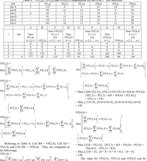
The value of VP(2,j), VP(3,j) and VP(4,j) in Table 4 are computed as the following:
[image:2.595.310.534.559.696.2]Table 4 : VP(2,j), VP(3,j) and VP(4,j) Computations for Job A as 5th Job Selection
Job j P(1,j) P(2,j) P(3,j) P(4,j) P(5,j) P(6,j)
Job A 5 135 8 6 41 14 31
Job B - 99 12 14 25 9 36
Job C 6 42 5 11 19 15 31
Job D - 91 13 14 39 4 16
Job E - 135 11 13 41 8 60
Job F - 101 10 11 31 12 59
A B C D E F G H K
j Job Sum
P(1,k)
k=2,j+1 VP(2,j)
Sum VP(2,k)
k=1,j-1 For
j=2,3…n-1 Sum
VP(2,k)
k=1,j VP(3,j)
Sum VP(3,k)
k=1,j-1 For
j=2,3..…n-1
Sum
VP(3,k)
k=1,j VP(4,j)
Sum VP(4,k)
k=1,j-1 For
j=2,3..…n-1
1 - 0 0 0 0 0 0
2 - 0 0 0 0 0 0 0 0 0
3 - 0 0 0 0 0 0 0 0 0
4 - 135 135 0 135 143 0 143 149 0 5 A 177 42 135 177 61 143 204 86 149
VP(2,j) =
∑
∑
∑
− = + = − = ⎥− ⎥ ⎦ ⎤ ⎢ ⎢ ⎣ ⎡ ⎥ ⎦ ⎤ ⎢ ⎣ ⎡ + ⎥ ⎦ ⎤ ⎢ ⎣ ⎡ 1 1 1 2 1 1 ) , 2 ( ) , 1 ( ), , 2 ( ) , 2 ( j k j k j k k VP k P j P k VP MaxVP(3,j) =
⎥ ⎥ ⎥ ⎥ ⎥ ⎦ ⎤ ⎢ ⎢ ⎢ ⎢ ⎢ ⎣ ⎡ + + + ⎥ ⎦ ⎤ ⎢ ⎣ ⎡ + + + + ⎥ ⎦ ⎤ ⎢ ⎣ ⎡
∑
∑
∑
∑
∑
− = = − = = = 1 1 5 4 1 1 5 3 1 ) , ( ) , 4 ( ) 1 , 3 ( ) 1 , 2 ( , ) , ( ) , 3 ( ) 1 , 2 ( ), 1 , 2 ( ) , 2 ( j k i j k i j k j i P k VP P P j i P k VP P j P k VP Max - ⎥ ⎦ ⎤ ⎢ ⎣ ⎡ +∑
− = 1 1 ) , 3 ( ) 1 , 2 ( j k k VP PVP(4,j) =
⎥ ⎦ ⎤ ⎢ ⎣ ⎡ + − ⎥ ⎥ ⎦ ⎤ ⎢ ⎢ ⎣ ⎡ ⎥ ⎦ ⎤ ⎢ ⎣ ⎡ + + + + ⎥ ⎦ ⎤ ⎢ ⎣ ⎡
∑
∑
∑
∑
− = − = = = 1 1 1 1 6 4 1 ) , 4 ( ) 1 , 3 ( ) , ( ) , 4 ( ) 1 , 3 ( ), 1 , 3 ( ) , 3 ( j k j k i j k k VP P j i P k VP P j P k VP MaxReferring to Table 4, Cell B4 = VP(2,4), Cell E4 =
VP(3,4) and Cell H4 = VP(4,4) . They are computed as the followings:
VP(2,4) =
∑
∑
∑
− = + = − = − ⎥ ⎦ ⎤ ⎢ ⎣ ⎡ ⎥ ⎦ ⎤ ⎢ ⎣ ⎡ + ⎥ ⎦ ⎤ ⎢ ⎣⎡ 41
1 1 4 2 1 4 1 ) , 2 ( ) , 1 ( ), 4 , 2 ( ) , 2 ( k k k k VP k P P k VP Max
= Max [{C4 + P(2,4)}, A4] - C4
= Max [{0 + 0}, 135] - 0 (P(2,4)=0 because j=4 has not yet been assigned) = 135
VP(3,4) =
⎥ ⎥ ⎥ ⎥ ⎦ ⎤ ⎢ ⎢ ⎢ ⎢ ⎣ ⎡ + + + ⎥ ⎦ ⎤ ⎢ ⎣ ⎡ + + + + ⎥ ⎦ ⎤ ⎢ ⎣ ⎡
∑
∑
∑
∑
∑
− = = − = = = 1 4 1 5 4 1 4 1 5 3 4 1 ) 4 , ( ) , 4 ( ) 1 , 3 ( ) 1 , 2 ( , ) 4 , ( ) , 3 ( ) 1 , 2 ( ), 1 4 , 2 ( ) , 2 ( k i k i k i P k VP P P i P k VP P P k VP Max - ⎥⎦ ⎤ ⎢⎣ ⎡ +∑
− = 1 4 1 ) , 3 ( ) 1 , 2 ( k k VP P= Max [{D4+P(2,5)},{P(2,1)+F4+P(3,4)+P(4,4)+P(5,4)}, {P(2,1) + P(3,1) + K4 + P(4,4) + P(5,4)}] - {P(2,1) + F4}
= Max [{135+8},{0+0+0+0+0},{0+0+0+0+0}]-{0+0} = 143
VP(4,4) =
⎥ ⎦ ⎤ ⎢ ⎣ ⎡ + − ⎥ ⎥ ⎥ ⎥ ⎥ ⎦ ⎤ ⎢ ⎢ ⎢ ⎢ ⎢ ⎣ ⎡ ⎥ ⎦ ⎤ ⎢ ⎣ ⎡ + + + + ⎥ ⎦ ⎤ ⎢ ⎣ ⎡
∑
∑
∑
∑
− = − = = = 1 4 1 1 4 1 6 4 4 1 ) , 4 ( ) 1 , 3 ( ) 4 , ( ) , 4 ( ) 1 , 3 ( ), 1 4 , 3 ( ) , 3 ( k k i k k VP P i P k VP P P k VP Max= Max [{G4 + P(3,5)}, {P(3,1) + K4 + P(4,4) + P(5,4) + P(6,4)}] - {P(3,1) + K4}
= Max [{143 + 6}, {0 + 0 + 0 + 0 + 0}] - {0 + 0} = 149
The value for VP(2,5), VP(3,5) and VP(4,5) can be computed using the similar approach as in the above description. Then the BAM4 index for Job A can be computed and its value equals to 42.The next move is to complete the computation of the 5th job BAM4 index for
other remaining jobs (i.e. Jobs B, D, E and F). The 5th job
BAM4 indexes for all the jobs is summarised in Table 5. Since there is no zero or negative BAM4 index value, therefore the positive values are to be considered. From this table, the smallest positive value for the BAM4 index belongs to Job D. Therefore, Job D is assigned as the 5th
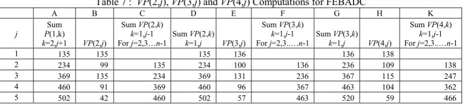
Table 7 : VP(2,j), VP(3,j) and VP(4,j) Computations for FEBADC
A B C D E F G H K
j PSum (1,k)
k=2,j+1 VP(2,j)
Sum VP(2,k) k=1,j-1 For j=2,3…n-1
Sum VP(2,k) k=1,j VP(3,j)
Sum VP(3,k) k=1,j-1 For j=2,3..…n-1
Sum VP(3,k) k=1,j VP(4,j)
Sum VP(4,k) k=1,j-1 For j=2,3..…n-1
1 135 135 135 136 136 138
2 234 99 135 234 100 136 236 109 138
3 369 135 234 369 131 236 367 115 247
4 460 91 369 460 96 367 463 104 362
5 502 42 460 502 57 463 520 59 466
With the assignment of Job D as the 5th job, the next
steps are to compute the BAM4 index for the 4th, 3rd, and
2nd job respectively (Step 5). The remaining job is
ultimately assigned to the 1st job. The recommended job
sequence by using BAM4 is therefore FEBADC. The makespan for this sequence can be computed using Equation 1. (Step 6). Using the process time data in Table 4 with FEBADC job scheduling, Table 7 is built to show the values of VP(2,j), VP(3,j) and VP(4,j) for determination of the P1BCF to be used in (1).
By using (3), the P1BCF for the FEBADC job arrangement can be computed as the followings:
P1BCF = Max
⎥ ⎥ ⎦ ⎤ ⎢
⎢ ⎣ ⎡
− −
+
∑
∑
∑
∑
= =
−
= =
n
j i n
j i
n i P j
P j
VP i
P
2
3
2 1
1 3
2
) , ( )
, 1 ( )
, 4 ( )
1 , ( , 0
(3) = Max [0,{P(2,1)+P(3,1)+VP(4,1)+VP(4,2)+VP(4,3)+ VP(4,4)+VP(4,5)}-{P(1,2)+P(1,3)+P(1,4)+P(1,5) +P(1,6)}- {P(2,6)+P(3,6)}]
= Max [0,{10+11+138+109+115+104+59}-{135+99+ 135 + 91 + 42}-{5 + 11}]
= Max [0, 546-502-16] = Max [0, 28] = 28
Therefore, by using (1) the makespan for the FEBADC job arrangement is computed as follows:
Makespan =
∑
∑
= =
+
n
j i
n
i
P
j
P
1
6
2
)
,
(
)
,
1
(
+ P1BCF= {P(1,1)+P(1,2)+P(1,3)+P(1,4)+P(1,5)+P(1,6)} +{P(2,6)+P(3,6)+P(4,6)+P(5,6)+P(6,6)}+P1BCF
={101+135+99+135+91+42}+{5+11+19+15+31}+28 = 603+81+28 = 712 hours
The next step in implementing BAM4 heuristic is the scheduling performance evaluation using the BSP4 index. This index is measured as the followings: (Step 7)
BSP4 index = P1BCF +
∑
=
6
2
)
,
(
i
n
i
P
(4)Therefore, for the FEBADC scheduling arrangement: BSP4 index = P1BCF+{P(2,6)+P(3,6)+P(4,6)+P(5,6)+ P(6,6)}
= 28+{5+11+19+15+31} = 109
From Table 2, it can be noted that the jobs other than Job C (assigned as the last job in the current schedule)
that are having
∑
=
6
2
)
,
(
ij
i
P
less than the current BSP4index of 109 are Job A, B and D. Therefore, new schedule
arrangements have to be established with Job A, B and D assigned as the last job candidates. By repeating Step 3 to 6 of BAM4 heuristic, the other recommended job sequences by using BAM4 index are FEDCBA, FEDCAB and FECBAD with makespan value 703, 699 and 689 hours respectively. As such, BAM4 heuristic will select FECBAD as its best scheduling solution (Step 8). This BAM4 heuristic result was verified by comparing its makespan value to the minimum makespan value obtained using complete enumeration. This enumeration is found resulting to a minimum makespan of 689 hours.
IV. BAM4 HEURISTIC PERFORMANCE EVALUATION
This section discusses the simulated results of the BAM4 heuristic performance under groups of weak, medium and strong dominance level values as described in [16]. The performance evaluation was first simulated using groups of 6 jobs waiting to be scheduled. The processing time for each process was randomly generated using uniform distribution pattern on the realistic data ranges as in Table 8. During each simulation, data on P1 dominance level, minimum makespan from BAM4 heuristic and minimum makespan from NEH heuristic (heuristic from Nawaz, Enscore and Ham as in [18]) were recorded. The ratio between BAM4 heuristic makespan and the NEH makespan was then computed for performance comparisons. A total of 3000 simulations were conducted. Table 9 shows the makespan performance comparison between BAM4 and NEH in solving the 6 job scheduling problem. It can be seen that BAM4 produces highest accuracy result at strong P1 dominance level. Since this study considers NEH as the best known heuristic for flow-shop scheduling as in [15,18] and appropriate tool for BAM4 performance verification, it can be highlighted that at strong P1 dominance level, BAM4 produced 93.55% + 0.3% or 93.85% accurate result. This dominance level also produced average BAM4 makespan performance of 0.1% above the NEH makespan.
Table 8 : Process Time Data Range (hours)
P(1,j)P(2,j) P(3,j) P(4,j) P(5,j)P(6,j)
Minimum 8 4 4 8 4 8
Table 9 : BAM4 vs NEH for 6 Job Problem
P1 Dominance
Level
Average BAM4/NEH
Ratio
BAM4 < NEH
(%)
BAM4 = NEH
(%)
BAM4 > NEH
(%) Weak 1.033702 0.816327 25.714286 73.469388 Medium 1.028987 0.325556 40.423223 59.251221 Strong 1.001006 0.299850 93.553223 6.146927
Overall 1.023536 0.4 49.833333 49.766667
[image:5.595.56.287.235.433.2]The BAM4 performance evaluation was also simulated using groups of 10 and 20 jobs. The simulation result analysis is presented in Table 10 and 11. These two tables show that at strong P1 dominance level BAM4 generates slightly better result compare to the NEH.
Table 10 : BAM4 vs NEH for 10 Job Problem
P1 Dominance
Level
Average BAM4/NEH
Ratio
BAM4 < NEH
(%)
BAM4 = NEH
(%)
BAM4 > NEH
(%)
Weak 1.029161 0 14.613527 85.386473
Medium 1.033239 3.383459 22.650376 73.966165 Strong 0.999512 8.935018 89.801444 1.263538
Overall 1.019657 4.5 45.233333 50.266667
Table 11 : BAM4 vs NEH for 20 Job Problem
P1 Dominance
Level
Average BAM4/NEH
Ratio
BAM4 < NEH (%)
BAM4 = NEH
(%)
BAM4 > NEH
(%)
Weak 1.019026 0 5.370844 94.62915
Medium 1.018700 1.35823 21.90152 76.74023 Strong 0.99998 0.96153 98.84615 0.192308 Overall 1.012295 0.86666 44.266667 54.866667
V. CONCLUSION
This research developed and evaluated a bottleneck-based scheduling heuristic of a four machine permutation re-entrant flow shop with the process routing of M1,M2,M3,M4,M3,M4. It was shown that at strong P1 dominance level, BAM4 heuristic is capable to produce near optimal results for all the problem sizes studied. Within strong P1 dominance level and at medium to high job numbers (n=10 and 20), this heuristic generates results which are very much compatible to the NEH. To some extent, in the specific 10 and 20 job problems simulation conducted during the study, BAM4 shows better average makespan compared to the NEH. However, for smaller job numbers (n=6), NEH is superior. The bottleneck approach presented in this paper can also be utilised to develop specific heuristics for other re-entrant and ordinary flow shop operation systems that shows significant bottleneck characteristics. With the successful development of the BAM4 heuristic, the next phase of this research is to further utilize the bottleneck approach in developing heuristic for the medium and weak P1 dominance level.
ACKNOWLEDGMENTS
This work was partially supported by the Fundamental Research Grant Scheme of Malaysia (Cycle 1 2007 Vot 0368).
REFERENCES
[1] Graves SC, Meal HC, Stefek D, Zeghmi AH (1983), “Scheduling of re-entrant flow shops”, Journal of Operations Management, Vol. 3(4), pp. 197-207
[2] Kubiak W, Lou SXC, Wang Y (1996), “Mean flow time minimization in reentrant job shops with a hub”, Operations Research, Vol. 44(5), pp. 764-776
[3] Hwang H, Sun JU (1997), ”Production sequencing problem with reentrant work flows and sequence dependent setup times”, Computers & Ind. Engng, Vol. 33(3-4), pp.773-776 [4] Wang MY, Sethi SP, Van de Velde SL (1997),”Minimizing
makespan in a class of reentrant shops”, Operations Research, Vol. 45(5), pp. 702-712
[5] Drobouchevitch IG, Strusevich VA (1999),”A heuristic algorithm for two-machine re-entrant shop scheduling”, Annals of Operations Research, Vol. 86(1), pp. 417-439 [6] Chen JS (2006),”A branch and bound procedure for the
reentrant permutation flow-shop scheduling problem”, Int. J Adv Manuf Technology, Vol. 19, pp. 1186-1193
[7] Choi SW, Kim YD (2007),”Minimizing makespan on a two-machine re-entrant flowshop”, Journal of the Operational Research Society, Vol. 58, pp. 972-981
[8] Demirkol E, Uzsoy R (2000), “Decomposition methods for reentrant flow shops with sequence dependent setup times”, Journal of Scheduling, Vol. 3, pp. 115-177
[9] Pan JC, Chen JS (2003), “Minimizing makespan in re-entrant permutation flow-shops”, Journal of Operation Research Society, Vol. 54, pp. 642-653
[10]Pearn WL, Chung SH, Chen AY, Yang MH (2004), “A case study on the multistage IC final testing scheduling problem with reentry”, International Journal of Production Economics, Vol. 88, pp. 257-267
[11]Choi SW, Kim YD, Lee GC, (2005), “Minimizing total tardiness of orders with reentrant lots in a hybrid flowshop”, International Journal of Production Research, Vol. 43, pp.2049-2067
[12]Choi SW, Kim YD (2008), “Minimizing makespan on an m -machine re-entrant flowshop”, Computers & Operations Research, Vol. 35(5), pp. 1684-1696
[13]Adams J, Balas E, Zawack D (1988), “The shifting bottleneck procedure for job shop scheduling”, Management Science, Vol. 34, pp. 391-401
[14]Mukherjee S, Chatterjee AK (2006), “Applying machine based decomposition in 2-machine flow shops”, European Journal of Operational Research, Vol. 169, pp. 723-741 [15]Kalir AA, Sarin SC (2001), “A near optimal heuristic for the
sequencing problem in multiple-batch flow-shops with small equal sublots”, The International Journal of Management Science (Omega), Vol. 29, pp. 577-584
[16]Bareduan SA, Hasan SH (2008b),”Bottleneck adjacent matching 3 (BAM3) heuristic for re-entrant flow shop with dominant machine”, submitted to the International Conference of Industrial Engineering and Engineering Management (IEEM2008), Singapore
[17] Bareduan SA, Hasan SH (2008a),”Makespan computation for cyber manufacturing centre using bottleneck analysis: a re-entrant flow shop problem“, in proc. of the International Multiconference of Engineers and Computer Scientist (IMECS 2008), Hong Kong, 19-21 March