R E S E A R C H
Open Access
Strong convergence of an
extragradient-type algorithm for the
multiple-sets split equality problem
Ying Zhao
†and Luoyi Shi
*†*Correspondence:
Department of Mathematics, Tianjin Polytechnic University, Tianjin, 300387, P.R. China
†Equal contributors
Abstract
This paper introduces a new extragradient-type method to solve the multiple-sets split equality problem (MSSEP). Under some suitable conditions, the strong convergence of an algorithm can be verified in the infinite-dimensional Hilbert spaces. Moreover, several numerical results are given to show the effectiveness of our algorithm.
Keywords: strong convergence; extragradient-type; multiple-sets split equality problem
1 Introduction
The split feasibility problem (SFP) was first presented by Censoret al.[]; it is an inverse problem that arises in medical image reconstruction, phase retrieval, radiation therapy treatment, signal processingetc. The SFP can be mathematically characterized by finding a pointxthat satisfies the property
x∈C, Ax∈Q, (.)
if such a point exists, whereCandQare nonempty closed convex subsets of Hilbert spaces HandH, respectively, andA:H→His a bounded and linear operator.
There are various algorithms proposed to solve the SFP, see [–] and the references therein. In particular, Byrne [, ] introduced the CQ-algorithm motivated by the idea of an iterative scheme of fixed point theory. Moreover, Censoret al.[] introduced an extension upon the form of SFP in with an intersection of a family of closed and convex sets instead of the convex setC, which is the original of the multiple-sets split feasibility problem (MSSFP).
Subsequently, an important extension, which goes by the name of split equality problem (SEP), was made by Moudafi []. It can be mathematically characterized by finding points x∈Candy∈Qthat satisfy the property
Ax=By, (.)
if such points exist, whereCandQare nonempty closed convex subsets of Hilbert spaces HandH, respectively,His also a Hilbert space,A:H→HandB:H→Hare two
bounded and linear operators. WhenB=I, the SEP reduces to SFP. For more information about the methods for solving SEP, see [, ].
This paper considers the multiple-sets split equality problem (MSSEP) which general-izes the MSSFP and SEP and can be mathematically characterized by finding pointsxand ythat satisfy the property
x∈ t
i=
Ci and y∈ r
j=
Qj such thatAx=By, (.)
where r,tare positive integers, {Ci}ti=∈H and{Qj}rj=∈H are nonempty, closed and
convex subsets of Hilbert spacesH andH, respectively,His also a Hilbert space,A: H →H, B:H→H are two bounded and linear operators. Obviously, ifB=I, the
MSSEP is just right MSSFP; ift=r= , the MSSEP changes into the SEP. Moreover, when B=Iandt=r= , the MSSEP reduces to the SFP.
One of the most important methods for computing the solution of a variational inequal-ity and showing the quick convergence is an extragradient algorithm, which was first in-troduced by Korpelevich []. Moreover, this method was applied for finding a common element of the set of solutions for a variational inequality and the set of fixed points of a nonexpansive mapping, see Nadezhkina et al.[]. Subsequently, Cenget al.in [] presented an extragradient method, and Yaoet al.in [] proposed a subgradient extra-gradient method to solve the SFP. However, all these methods to solve the problem have only weak convergence in a Hilbert space. On the other hand, a variant extragradient-type method and a subgradient extragradient method introduced by Censoret al.[, ] possess strong convergence for solving the variational inequality.
Motivated and inspired by the above works, we introduce an extragradient-type method to solve the MSSEP in this paper. Under some suitable conditions, the strong convergence of an algorithm can be verified in the infinite-dimensional Hilbert spaces. Finally, several numerical results are given to show the feasibility of our algorithm.
2 Preliminaries
LetHbe a real Hilbert space whose inner product and norm are denoted by·,·and · , respectively. LetIdenote the identity operator onH.
Next, we recall several definitions and basic results that will be available later.
Definition . A mappingT:H→Hgoes by the name of
(i) nonexpansive if
Tx–Ty ≤ x–y, ∀x,y∈H;
(ii) firmly nonexpansive if
Tx–Ty ≤ x–y,Tx–Ty, ∀x,y∈H;
(iii) contractive onxif there exists <α< such that
(iv) monotone if
Tx–Ty,x–y ≥, ∀x,y∈H;
(v) β-inverse strongly monotone if there existsβ> such that
Tx–Ty,x–y ≥βTx–Ty, ∀x,y∈H.
The following properties of an orthogonal projection operator were introduced by Bauschkeet al.in [], and they will be powerful tools in our analysis.
Proposition .([]) Let PCbe a mapping from H onto a closed,convex and nonempty subset C of H if
PC(x) =arg min
y∈Cx–y, ∀x∈H,
then PCis called an orthogonal projection from H onto C.Furthermore,for any x,y∈H and z∈C,
(i) x–PCx,z–PCx ≤;
(ii) PCx–PCy≤ PCx–PCy,x–y;
(iii) PCx–z≤ x–z–PCx–x.
The following lemmas provide the main mathematical results in the sequel.
Lemma .([]) Let C be a nonempty closed convex subset of a real Hilbert space H,let
T:C→H beα-inverse strongly monotone,and let r> be a constant.Then,for anyx,y∈ C,
(I–rT)x– (I–rT)y≤ x–y+r(r– α)T(x) –T(y).
Moreover, when <r< α,I–rTis nonexpansive.
Lemma .([]) Let{xk}and{yk}be bounded sequences in a Hilbert space H,and let{β k} be a sequence in[, ]which satisfies the condition <lim infk→∞βk≤lim supk→∞βk< . Suppose that xk+= (–βk)yk+β
kxkfor all k≥andlim supk→∞(yk+–yk–xk+–xk)≤ .Thenlimk→∞yk–xk= .
The lemma below will be a powerful tool in our analysis.
Lemma .([]) Let{ak}be a sequence of nonnegative real numbers satisfying the condi-tion ak+≤( –mk)ak+mkδk,∀k≥,where{mk},{δk}are sequences of real numbers such that
(i) {mk} ∈[, ]and ∞
k=mk=∞or,equivalently, ∞
k=
( –mk) = lim k→∞
k
j=
(ii) lim supk→∞δk≤or
(ii)’ ∞k=δkmkis convergent.Thenlimk→∞ak= .
3 Main results
In this section, we propose a formal statement of our present algorithm. Review the multiple-sets split equality problem (MSSEP), without loss of generality, suppose t>r in (.) and defineQr+=Qr+=· · ·=Qt=H. Hence, MSSEP (.) is equivalent to the
following problem:
find x∈ t
i=
Ci and y∈ t
j=
Qj such thatAx=By. (.)
Moreover, setSi=Ci×Qi∈H=H×H(i= , , . . . ,t),S=
t
i=Si,G= [A, –B] :H→ H, the adjoint operator ofGis denoted byG∗, then the original problem (.) reduces to
finding w= (x,y)∈S such thatGw= . (.)
Theorem . Let=∅be the solution set of MSSEP(.).For an arbitrary initial point w∈S,the iterative sequence{wn}can be given as follows:
⎧ ⎨ ⎩
vn=PS{( –αn)wn–γnG∗Gwn}, wn+=PS{wn–μnG∗Gvn+λn(vn–wn)},
(.)
where {αn}∞n= is a sequence in [, ] such that limn→∞αn = ,and ∞
n=αn =∞, and
{γn}∞n=,{λn}∞n=,{μn}∞n=are sequences in H satisfying the following conditions:
⎧ ⎪ ⎪ ⎪ ⎪ ⎪ ⎨ ⎪ ⎪ ⎪ ⎪ ⎪ ⎩
γn∈(,ρ(G∗G)), limn→∞(γn+–γn) = ;
λn∈(, ), limn→∞(λn+–λn) = ;
μn≤ρ(G∗G)λn, limn→∞(μn+–μn) = ;
∞ n=(
γn λn) <∞.
(.)
Then{wn}converges strongly to a solution of MSSEP(.).
Proof In view of the property of the projection, we inferwˆ=PS(wˆ –tG∗Gwˆ) for anyt> . Further, from the condition in (.), we get thatμn≤ρ(G∗G)λn, it follows thatI–
μn λnG
∗G
is nonexpansive. Hence,
wn+–wˆ
=PS
wn–μnG∗Gvn+λn(vn–wn)
–PS
ˆ
w–tG∗Gwˆ =PS
( –λn)wn+λn
I–μn λn
G∗G
vn
–PS
( –λn)wˆ+λn
I–μn λn
G∗G
ˆ
w
≤( –λn)wn–wˆ+λn I–μn
λn G∗G
vn–
I–μn
λn G∗G
ˆ
w
Sinceαn→ asn→ ∞and from the condition in (.),γn∈(,ρ(G∗G)), it follows that
αn≤ –γnρ(G
∗G)
asn→ ∞, that is,
γn –αn ∈(,
ρ(G∗G)). We deduce that
vn–wˆ =PS
( –αn)wn–γnG∗Gwn
–PS
ˆ
w–tG∗Gwˆ
≤( –αn)
wn– γn –αn
G∗Gwn
–
αnwˆ + ( –αn)
ˆ
w– γn –αn
G∗Gwˆ
≤–αnwˆ+ ( –αn)
wn– γn –αn
G∗Gwn–wˆ + γn –αn
G∗Gwˆ, (.)
which is equivalent to
vn–wˆ ≤αn–wˆ+ ( –αn)wn–wˆ. (.)
Substituting (.) in (.), we obtain
wn–wˆ ≤( –λn)wn–wˆ+λn
αn–wˆ+ ( –αn)wn–wˆ
≤( –λnαn)wn–wˆ+λnαn–wˆ
≤maxwn–wˆ,–wˆ
.
By induction,
wn–wˆ ≤max
w–wˆ,–wˆ
.
Consequently,{wn}is bounded, and so is{vn}.
LetT= PS–I. From Proposition ., one can know that the projection operatorPSis monotone and nonexpansive, and PS–Iis nonexpansive.
Therefore,
wn+= I+T
( –λn)wn+λn
–μn λn
G∗G
vn
=I–λn wn+
λn
I–μn
λn G∗G
vn+
T
( –λn)wn+λn
I–μn λn
G∗G
vn
,
that is,
wn+=
–λn wn+
+λn
bn, (.)
wherebn=
λn(I–μλnnG∗G)vn+T[(–λn)wn+λn(I–
μn
λnG∗G)vn]
+λn .
Indeed,
bn+–bn
≤ λn+
+λn+
I–μn+ λn+
G∗G
vn+–
I–μn
λn G∗G
vn
+ λn+ +λn+
– λn +λn
×
I–μn
λn G∗G
vn
+ T
+λn+
( –λn+)wn++λn+
I–μn+
λn+ G∗G
vn+
–
( –λn)wn+λn
I–μn λnG
∗Gv n
+
+λn+
–
+λn
×T
( –λn)wn+λn
I–μn λn
G∗G
vn
. (.)
For convenience, letcn= (I– μλnnG
∗G)v
n. By Lemma . in Shiet al.[], it follows that (I–μn
λnG
∗G) is nonexpansive and averaged. Hence,
bn+–bn
≤ λn+
+λn+
cn+–cn+ λn+
+λn+
– λn +λn
cn
+ T
+λn+
( –λn+)wn++λn+cn+–
( –λn)wn+λncn
+ +λn+
–
+λn
T( –λn)wn+λncn
≤ λn+
+λn+
cn+–cn+ λn+
+λn+
– λn +λn
cn
+ –λn+ +λn+
wn+–wn+ λn+
+λn+
cn+–cn+
λn–λn+
+λn+ wn
+λn+–λn +λn+
cn+
+λn+ – +λn
T( –λn)wn+λncn. (.)
Moreover,
cn+–cn =
I–μn+
λn+ G∗G
vn+–
I–μn
λn G∗G
vn
≤ vn+–vn =PS
( –αn+)wn+–γnG∗Gwn+
–PS
( –αn)wn–γnG∗Gwn
≤I–γn+G∗G
wn+–
I–γn+G∗G
wn+ (γn–γn+)G∗Gwn
+αn+–wn++αnwn
≤ wn+–wn+|γn–γn+|G∗Gwn+αn+–wn++αnwn. (.)
Substituting (.) in (.), we infer that
bn+–bn
≤ λn+
+λn+
– λn +λn
cn+
λn–λn+
+λn+
wn+
λn+–λn +λn+
cn
+wn+–wn+
+λn+ – +λn
T( –λn)wn+λncn
By virtue oflimn→∞(λn+–λn) = , it follows thatlimn→∞|+λλn+n+–
λn
+λn|= . Moreover,
{wn}and{vn}are bounded, and so is{cn}. Therefore, (.) reduces to
lim sup
n→∞
bn+–bn–wn+–wn
≤. (.)
Applying (.) and Lemma ., we get
lim
n→∞bn–wn= . (.)
Combining (.) with (.), we obtain
lim
n→∞xn+–xn= .
Using the convexity of the norm and (.), we deduce that
wn+–wˆ
≤( –λn)wn–wˆ+λnvn–wˆ
≤( –λn)wn–wˆ+λn –αnwˆ
+ ( –αn)
wn– γn –αn
G∗Gwn–
ˆ
w– γn –αn
G∗Gwˆ
≤( –λn)wn–wˆ+λnαn–wˆ + ( –αn)λn
wn–wˆ+ γn –αn
γn –αn–
ρ(G∗G)
G∗Gwn–G∗Gwˆ
≤ wn–wˆ+λnαn–wˆ+λnγn
γn –αn
–
ρ(G∗G)
G∗Gwn–G∗Gwˆ
,
which implies that
λnγn
ρ(G∗G)–
γn –αn
G∗Gwn–G∗Gwˆ
≤ wn–wˆ–wn+–wˆ+λnαn–wˆ
≤ wn+–wn
wn–wˆ+wn+–wˆ
+λnαn–wˆ.
Sincelim infn→∞λnγn(ρ(G∗G)–
γn
–αn) > ,limn→∞αn= andlimn→∞wn+–wn= , we infer that
lim
n→∞G ∗Gw
n–G∗Gwˆ= . (.)
Applying Proposition . and the property of the projectionPS, one can easily show that
vn–wˆ =PS
( –αn)wn–γnG∗Gwn
–PS
ˆ
w–γnG∗Gwˆ
≤( –αn)wn–γnG∗Gwn–
ˆ
w–γnG∗Gwˆ
,vn–wˆ
=
wn–γnG ∗Gw
n–
ˆ
w–γnG∗Gwˆ
–αnwn
+vn–wˆ –( –αn)wn–γnG∗Gwn–
ˆ
w–γnG∗Gwˆ
–vn+wˆ
≤
wn–wˆ+ αn–wnwn–γnG∗Gwn–
ˆ
w–γnG∗Gwˆ
–αnwn
+vn–wˆ–wn–vn–γnG∗G(wn–wˆ) –αnwn
≤
wn–wˆ+αnM+vn–wˆ–wn–vn + γn
wn–vn,G∗G(wn–wˆ)
+ αnwn,wn–vn–γnG∗G(wn–wˆ) +αnwn
≤
wn–wˆ+αnM+vn–wˆ
–wn–vn+ γnwn–vnG∗G(wn–wˆ) + αnwnwn–vn
≤ wn–wˆ+αnM–wn–vn+ γnwn–vnG∗G(wn–wˆ)
+ αnwnwn–vn, (.)
whereM> satisfies
M≥sup
k
–wnwn–γnG∗Gwn–
ˆ
w–γnG∗Gwˆ
–αnwn.
From (.) and (.), we get
wn+–wˆ
≤( –λn)wn–wˆ+λnvn–wˆ
≤ wn–wˆ–λnwn–vn+αnM+ γnwn–vnγnG∗G(wn–wˆ) + αnwnwn–vn,
which means that
λnwn–vn≤ wn+–wn
wn–wˆ+wn+–wˆ
+αnM
+ γnwn–vnγnG∗G(wn–wˆ) + αnwnwn–vn.
Sincelimn→∞αn= ,limn→∞wn+–wn= andlimn→∞G∗Gwn–G∗Gwˆ= , we infer that
lim
Finally, we show thatwn→ ˆw. Using the property of the projectionPS, we derive
vn–wˆ =PS
( –αn)
wn–
γn –αnG
∗Gw n
–PS
αnwˆ+ ( –αn)
ˆ
w– γn –αn
G∗Gwˆ
≤
( –αn)
I– γn
–αn G∗G
(wn–wˆ) –αnwˆ,vn–wˆ
≤( –αn)wn–wˆvn–wˆ+αn ˆw,wˆ–vn
≤ –αn
wn–wˆ+vn–wˆ
+αn ˆw,wˆ–vn, which equals
vn–wˆ≤ –αn +αn
wn–wˆ+ αn –αn ˆ
w,wˆ –vn. (.)
It follows from (.) and (.) that
wn+–wˆ
≤( –λn)wn–wˆ+λnvn–wˆ
≤( –λn)wn–wˆ+λn
–αn +αn
wn–wˆ+ αn –αn
ˆw,wˆ–vn
≤
–αnλn +αn
wn–wˆ+ αnλn –αn ˆ
w,wˆ–vn. (.)
Since γn –αn∈(,
ρ(G∗G)), we observe thatαn∈(, –
γnρ(G∗G) ), then
αnλn –αn
∈
,λn( –γnρ(G ∗G))
γnρ(G∗G)
,
that is to say,
αnλn –αn ˆ
w,wˆ–vn ≤
λn( –γnρ(G∗G)) γnρ(G∗G) ˆ
w,wˆ–vn.
By virtue of ∞n=(λn
γn) < ∞, γn ∈ (,
ρ(G∗G)) and ˆw,wˆ –vn is bounded, we obtain
∞ n=(
λn(–γnρ(G∗G))
γnρn(G∗G) ) ˆw,wˆ–vn<∞, which implies that
∞
n=
αnλn –αn
ˆw,wˆ –vn ≤ ∞.
Moreover,
∞
n=
αnλn –αn ˆ
w,wˆ –vn= ∞
n=
αnλn +αn
+αn –αn ˆ
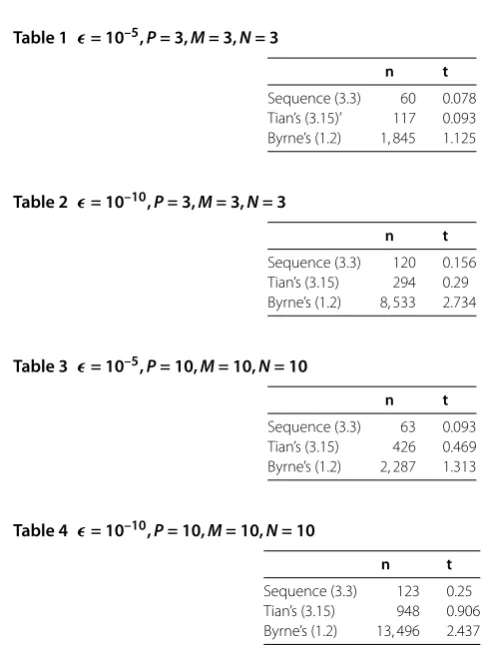
Table 1 = 10–5,P= 3,M= 3,N= 3
n t
Sequence (3.3) 60 0.078 Tian’s (3.15)’ 117 0.093 Byrne’s (1.2) 1, 845 1.125
Table 2 = 10–10,P= 3,M= 3,N= 3
n t
Sequence (3.3) 120 0.156 Tian’s (3.15) 294 0.29 Byrne’s (1.2) 8, 533 2.734
Table 3 = 10–5,P= 10,M= 10,N= 10
n t
Sequence (3.3) 63 0.093 Tian’s (3.15) 426 0.469 Byrne’s (1.2) 2, 287 1.313
Table 4 = 10–10,P= 10,M= 10,N= 10
n t
Sequence (3.3) 123 0.25 Tian’s (3.15) 948 0.906 Byrne’s (1.2) 13, 496 2.437
it follows that all the conditions of Lemma . are satisfied. Combining (.), (.) and Lemma ., we can show thatwn→ ˆw. This completes the proof.
4 Numerical experiments
In this section, we provide several numerical results and compare them with Tian’s [] algorithm (.)’ and Byrne’s [] algorithm (.) to show the effectiveness of our pro-posed algorithm. Moreover, the sequence given by our algorithm in this paper has strong convergence for the multiple-sets split equality problem. The whole program was writ-ten in Wolfram Mathematica (version .). All the numerical results were carried out on a personal Lenovo computer with Intel(R)Pentium(R) N CPU . GHz and RAM . GB.
In the numerical results,A= (aij)P×N,B= (bij)P×M, whereaij∈[, ],bij∈[, ] are all given randomly,P,M,N are positive integers. The initial pointx= (, , . . . , ), andy=
(, , . . . , ),αn= .,λn= .,γn= ρ(G.∗G),μn= ρ(G.∗G) in Theorem .,ρn=ρn = . in
Tian’s (.)’ andγn= . in Byrne’s (.). The termination condition isAx–By< . In Tables -, the iterative steps and CPU are denoted bynandt, respectively.
Competing interests
The authors declare that there are no competing interests.
Authors’ contributions
All authors contributed equally and significantly in writing this paper. All authors read and approved the final manuscript.
Acknowledgements
Received: 23 December 2016 Accepted: 20 February 2017 References
1. Censor, Y, Elfving, T: A multiprojection algorithm using Bregman projections in a product space. Numer. Algorithms 8(2-4), 221-239 (1994)
2. Xu, HK: A variable Krasnosel’skii-Mann algorithm and the multiple-set split feasibility problem. Inverse Probl.22(6), 2021-2034 (2006)
3. Lopez, G, Martin-Marqnez, V, Wang, F, Xu, HK: Solving the split feasibility problem without prior knowledge of matrix norms. Inverse Probl.28, 085004 (2012)
4. Yang, Q: The relaxed CQ algorithm solving the split feasibility problem. Inverse Probl.20(4), 1261-1266 (2004) 5. Byrne, C: Iterative oblique projection onto convex sets and the split feasibility problem. Inverse Probl.18(2), 441-453
(2002)
6. Byrne, C: A unified treatment of some iterative algorithms in signal processing and image reconstruction. Inverse Probl.20(1), 103-120 (2004)
7. Censor, Y, Elfving, T, Kopf, N, Bortfeld, T: The multiple-sets split feasibility problem and its applications for inverse problems. Inverse Probl.21(6), 2071-2084 (2005)
8. Moudafi, A: Alternating CQ algorithm for convex feasibility and split fixed point problem. J. Nonlinear Convex Anal. 15(4), 809-818 (2013)
9. Shi, LY, Chen, RD, Wu, YJ: Strong convergence of iterative algorithms for solving the split equality problems. J. Inequal. Appl.2014, Article ID 478 (2014)
10. Dong, QL, He, SN, Zhao, J: Solving the split equality problem without prior knowledge of operator norms. Optimization64(9), 1887-1906 (2015)
11. Korpelevich, GM: An extragradient method for finding saddle points and for other problems. Ekonomikai Matematicheskie Metody12(4), 747-756 (1976)
12. Nadezhkina, N, Takahashi, W: Weak convergence theorem by an extragradient method for nonexpansive mappings and monotone mappings. J. Optim. Theory Appl.128(1), 191-201 (2006)
13. Ceng, LC, Ansari, QH, Yao, JC: An extragradient method for solving split feasibility and fixed point problems. Comput. Math. Appl.64(4), 633-642 (2012)
14. Yao, Y, Postolache, M, Liou, YC: Variant extragradient-type method for monotone variational inequalities. Fixed Point Theory Appl.2013, Article ID 185 (2013)
15. Censor, Y, Gibali, A, Reich, S: The subgradient extragradient method for solving variational inequalities in Hilbert space. J. Optim. Theory Appl.148(2), 318-335 (2011)
16. Censor, Y, Gibali, A, Reich, S: Strong convergence of subgradient extragradient method for the variational inequalities in Hilbert space. Optim. Methods Softw.26(4-5), 827-845 (2011)
17. Bauschke, HH, Combettes, PL: Convex Analysis and Monotone Operator Theory in Hilbert Space. Springer, London (2011)
18. Takahashi, W, Toyoda, M: Weak convergence theorems for nonexpansive mappings and monotone mappings. J. Optim. Theory Appl.118(2), 417-428 (2003)
19. Suzuki, T: Strong convergence theorems for infinite families of nonexpansive mappings in general Banach spaces. Fixed Point Theory Appl.2005685918 (2005)
20. Xu, HK: Iterative algorithms for nonlinear operators. J. Lond. Math. Soc.66(1), 240-256 (2002)
21. Tian, D, Shi, L, Chen, R: Iterative algorithm for solving the multiple-sets split equality problem with split self-adaptive step size in Hilbert spaces. Arch. Inequal. Appl.2016(1), 1-9 (2016)