R E S E A R C H
Open Access
Smoothing of the lower-order exact
penalty function for inequality constrained
optimization
Shujun Lian
*and Yaqiong Duan
*Correspondence:
[email protected] College of Management, Qufu Normal University, Rizhao, Shandong 276826, China
Abstract
In this paper, we propose a method to smooth the general lower-order exact penalty function for inequality constrained optimization. We prove that an approximation global solution of the original problem can be obtained by searching a global solution of the smoothed penalty problem. We develop an algorithm based on the smoothed penalty function. It is shown that the algorithm is convergent under some mild conditions. The efficiency of the algorithm is illustrated with some numerical examples.
Keywords: inequality constrained optimization; exact penalty function; lower-order
penalty function; smoothing method
1 Introduction
We consider the following nonlinear constrained optimization problem:
[P] minf(x)
s.t.gi(x)≤, i= , , . . . ,m,
wheref :Rn→Randg
i:Rn→R,i∈I={, , . . . ,m}are twice continuously differentiable
functions. Let
G=
x∈Rn|gi(x)≤,i= , , . . . ,m
.
The penalty function methods have been proposed to solve problem [P] in much of the literature. In Zangwill [], the classicallexact penalty function is defined as follows:
p(x,q) =f(x) +q
m
i=
maxgi(x),
, (.)
whereq> is a penalty parameter, but it is not a smooth function. Differentiable approxi-mations to the exact penalty function have been obtained in various places in the literature, such as [–].
Recently lower-order penalty functions have been proposed in some literature. In [], Luo gave a global exact penalty result for a lower-order penalty function of the form
f(x) +α
m
i=
maxgi(x),
/γ
, (.)
whereα> ,γ ≥ are the penalty parameters. Obviously, it is thelpenalty function when
γ = .
The nonlinear penalty function has been investigated in [] and [] as follows:
Lk(x,d) =
f(x)k+
m
i= di
maxgi(x), k
/k
, (.)
wheref(x) is assumed to be positive,k> is a given number, andd= (d,d, . . . ,dm)∈Rm+ is the penalty parameter. It was shown in [] that the exact penalty parameter correspond-ing tok∈(, ] is substantially smaller than that of the classicallexact penalty function.
In [], the lower-order penalty functions
ϕq,k(x) =f(x) +q m
i=
maxgi(x), k
, k∈(, ), (.)
have been introduced and shown to be exact under some conditions, but its smoothing does not discussed fork∈(, ). Whenk=
, we have the following function:
ϕq(x) =f(x) +q m
i=
maxgi(x),
. (.)
Its smoothing has been investigated in [, ] and []. The smoothing of the lower-order exact penalty function (.) has been investigated in [] and [].
In this paper, we aim to smooth the lower-order penalty function (.). The rest of this paper is organized as follows. In Section , a new smoothing function to the lower-order penalty function (.) is introduced. The error estimates are obtained among the opti-mal objective function values of the smoothed penalty problem, the nonsmooth penalty problem and the original problem. In Section , we present an algorithm to compute an approximate solution to [P] based on the smooth penalty function and show that it is glob-ally convergent. In Section , three numerical examples are given to show the efficiency of the algorithm. In Section , we conclude the paper.
2 Smoothing exact lower-order penalty function We consider the following lower-order penalty problem:
[LOP]k min x∈Rnϕq,k(x).
Assumption f(x) satisfies the following coercive condition:
lim
x→+∞f(x) = +∞.
Under Assumption , there exists a boxXsuch thatG([P])⊂int(X), whereG([P]) is the set of global minima of problem [P],int(X) denotes the interior of the setX. Consider the following problem:
P
minf(x)
s.t.gi(x)≤, i= , , . . . ,m,
x∈X.
LetG([P]) denote the set of global minima of problem [P]. ThenG([P]) =G([P]).
Assumption The setG([P]) is a finite set.
Then for anyk∈(, ), we consider the penalty problem of the form
LOPk min x∈Xϕq,k(x).
We know that the lower-order penalty functionϕq,k(x)(k∈(, )) is an exact penalty
func-tion in [] under Assumpfunc-tion and Assumpfunc-tion . But the lower-order exact penalty functionϕq,k(x) (k∈(, )) is a nondifferentiable function. Now we consider its
smooth-ing.
Letpk(u) = (max{u, })k, that is,
pk(u) =
uk ifu> ,
otherwise, (.)
then
ϕq,k(x) =f(x) +q m
i= pk
gi(x). (.)
For any> , let
p,k(u) =
⎧ ⎪ ⎨ ⎪ ⎩
ifu≤,
–kuk if <u≤, uk–k
ifu>.
(.)
It is easy to see thatp,k(u) is continuously differentiable onR. Furthermore, we see that
p,k(u)→pk(u) as→.
Figure shows the behavior ofp/(u) (represented by the solid line),p.,/(u) (repre-sented by the dot line),p.,/(u) (represented by the broken line) andp.,/(u) (repre-sented by the dash and dot line).
Let
ϕq,,k(x) =f(x) +q m
i= p,k
Figure 1 The behavior ofp,2/3(u) andp2/3(u).
Thenϕq,,k(x) is continuously differentiable onRn. Consider the following smoothed
op-timization problem:
[SP] min
x∈Xϕq,,k(x).
Lemma . For any x∈X,> ,we see that
≤ϕq,k(x) –ϕq,,k(x)≤
mq
k.
Proof Note that
pk
gi(x) –p,k
gi(x) =
⎧ ⎪ ⎨ ⎪ ⎩
ifgi(x)≤,
(gi(x))k––k(gi(x))k if <gi(x)≤, k
ifgi(x) >.
Let
F(u) =uk–
–kuk.
We get
F(u) =kuk––k–kuk–=k–kuk–k–uk .
Whenu∈(,),F(u)≥. It is easy to see thatF(u) is monotone increasing in [,]. Whengi(x)∈[,], we can get
≤pk
gi(x) –p,k
gi(x) <
Thus we see that
≤ϕq,k(x) –ϕq,,k(x)≤
mq
k.
This completes the proof.
Theorem . Let{j} →+ be a sequence of positive numbers and assume that xj is a
solution tominx∈Xϕq,j,k(x)for some q> ,k∈(, ).Letx be an accumulation point of the¯
sequence{xj}.Thenx is an optimal solution to¯ minx∈Xϕq,k(x).
Proof Becausexjis a solution tominx∈Xϕq,j,k(x), we see that
ϕq,j,k(xj)≤ϕq,j,k(x), ∀x∈X.
By Lemma ., we see that
ϕq,j,k(x)≤ϕq,k(x)
and
ϕq,k(x)≤ϕq,j,k(x) +
mq
k j.
It follows that
ϕq,k(xj)≤ϕq,j,k(xj) +
mq
k
j ≤ϕq,j,k(x) +
mq
k
j ≤ϕq,k(x) +
mq
k j.
Letj→ ∞, we see that
ϕq,k(x¯)≤ϕq,k(x).
This completes the proof.
Theorem . Let x∗q,k∈X be an optimal solution of problem[LOP]kandx¯q,,k∈X be an
optimal solution of problem[SP]for some q> ,k∈(, )and> .Then we see that
≤ϕq,k
x∗q,k –ϕq,,k(x¯q,,k)≤
mq
k.
Proof By Lemma ., we see that
≤ϕq,k
x∗q,k –ϕq,,k
x∗q,k
≤ϕq,k
x∗q,k –ϕq,,k(x¯q,,k)
≤ϕq,k(x¯q,,k) –ϕq,,k(x¯q,,k)
≤
mq
k.
Theorem . and Theorem . mean that an approximately optimal solution to [SP] is also an approximately optimal solution to [LOP]kwhen the erroris sufficiently small.
Definition . For> , a pointx∈Xis an-feasible solution or an-solution of prob-lem [P], if
gi(x)≤, i= , , . . . ,m.
We say that the pair (x∗,λ∗) satisfies the second-order sufficiency condition in [] if
∇xL
x∗,λ∗ = ,
gi
x∗ ≤, i= , , . . . ,m,
λ∗i ≥, i= , , . . . ,m,
λ∗igi
x∗ = , i= , , . . . ,m,
yT∇Lx∗,λ∗ y> , for anyy∈Vx∗ ,
(.)
whereL(x,λ) =f(x) +mi=λigi(x), and
Vx∗ =y∈Rn|∇Tgi
x∗ y= ,i∈Ax∗ ;∇Tgi
x∗ y≤,i∈Bx∗ , Ax∗ =i∈ {, , . . . ,m}|gi
x∗ = ,λ∗> ,
Bx∗ =i∈ {, , . . . ,m}|gi
x∗ = ,λ∗= .
Theorem . Suppose that Assumptionsandhold,and that for any x∗∈G([P]),there exists aλ∗∈Rm
+ such that the pair(x∗,λ∗)satisfies the second-order sufficiency condition (.).Then for∀k∈(, ),let x∗∈X be a global solution of problem[P]andx¯q,,k∈X be
a global solution of problem[SP]for k∈(, ),> .Then there exists q∗> such that for any q>q∗,
≤fx∗ –ϕq,,k(x¯q,,k)≤
mq
k. (.)
Furthermore,ifx¯q,,kbe an-feasible solution of problem[P],then we see that
≤fx∗q,k –f(x¯q,,k)≤mqk,
where q∗> is defined in Corollary.in[].
Proof By Corollary . in [], we see thatx∗∈Xis a global solution of problem [LOP]k.
Then by Theorem ., we see that
≤ϕq,k
x∗ –ϕq,,k(x¯q,,k)≤
mq
k. (.)
Sincemi=pk(gi(x∗)) = , we have
ϕq,k
x∗ =fx∗ +q
m
i= pk
gi
By (.) and (.), we see that (.) holds. Furthermore, it follows from (.) and (.) that
≤fx∗ –
f(x¯q,,k) +q m
i= p,k
gi(x¯q,,k)
≤
mq
k.
It follows that
q
m
i= p,k
gi(x¯q,,k) ≤f
x∗ –f(x¯q,,k)≤
mq
k+q m
i= p,k
gi(x¯q,,k). (.)
From (.) and the fact thatx¯q,,kis an-feasible solution of problem [P], we see that
≤
m
i= p,k
gi(x¯q,,k) ≤
m
k. (.)
Then it follows from (.) and (.) that
≤fx∗ –f(x¯q,,k)≤mqk.
This completes the proof.
Theorem . means that an approximately optimal solution to [SP] is an approximately optimal solution to [P] if the solution to [SP] is-feasible.
3 A smoothing method
We propose the following algorithm to solve [P].
Algorithm .
Step Choose an initial pointx, and a stoping tolerance> . Given> ,q> , <
η< , andσ> , letj= and go to Step .
Step Usexjas the starting point to solveminx∈Rnϕq
j,j,k(x). Letx∗j be the optimal solution
obtained (x∗j is obtained by a quasi-Newton method and a finite difference gradient). Step Ifx∗j is-feasible to [P], then stop and we have obtained an approximately optimal solutionx∗j of the original problem [P]. Otherwise, letqj+=σqj,j+=ηj,xj+=x∗j, and
j=j+ , then go to Step .
From <η< andσ> , we can easily see that the sequence{j}is decreasing to and
the sequence{qj}is increasing to +∞asj−→+∞.
Now we prove the convergence of the algorithm under some mild conditions.
Theorem . Suppose that Assumptionholds and for any q∈[q, +∞),∈(,],the set
arg min
x∈Rnϕq,,k(x)=∅.
Let{x∗j}be the sequence generated by Algorithm..If the sequence{ϕqj,j,k(x∗j)}is bounded,
Proof First we show that{x∗j}is bounded. Note that
ϕqj,j,k
x∗j =fx∗j +qj m
i= pj,k
gi
x∗j , j= , , , . . . .
By the assumptions, there is some numberLsuch that
L>ϕqj,j,k
x∗j , j= , , , . . . .
Suppose to the contrary that {x∗j}is unbounded. Without loss of generality, we assume thatx∗j → ∞asj→ ∞. Then we get
L>fx∗j , j= , , , . . . ,
which results in a contradiction sincef is coercive.
We show next that any limit point of{x∗j}is the optimal solution of [P]. Letx¯be any limit point of{x∗j}. Then there exists a natural number setJ⊆N, such thatx∗j → ¯x,j∈J. If we can prove that (i)x¯∈Gand (ii)f(x¯)≤infx∈Gf(x) hold, thenx¯is the optimal solution of [P].
(i) Suppose to the contrary thatx¯∈/G, then there existδ> ,i∈Iand the subsetJ⊂J such that
gi
x∗j ≥δ>j
for anyj∈J.
And by step in Algorithm . and (.), we see that
fx∗j + qjδ
k
≤f
x∗j +qj
gi
x∗j k–
k j
≤ϕqj,j,k
x∗j ≤ϕqj,j,k(x) =f(x)
for anyx∈G, which contradicts withqj→+∞. Then we see thatx¯∈G.
(ii) For anyx∈G, we have
fx∗j ≤ϕqj,j,k
x∗j ≤ϕqj,j,k(x) =f(x),
thenf(x¯)≤infx∈Gf(x) holds.
This completes the proof.
4 Numerical examples
In this section, we solve three numerical examples to show the applicability of Algo-rithm ..
Example .(Example . in [], Example . in [] and Example . in [])
minf(x) =x+x–cos(x) –cos(x) + ,
Table 1 Numerical results for Example 4.1 withk= 1/3
j xj∗ qj j g1(xj∗) g2(xj∗) f (x∗j)
0 –0.362270 0.366667
1 0.1 3.154764 –0.224317 1.277367
1 0.724975 0.399152
2 0.01 –0.774989 –0.000000 1.837569
Table 2 Numerical results for Example 4.1 withk= 2/3
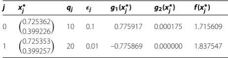
j x∗j qj j g1(xj∗) g2(x∗j) f (xj∗)
0 0.725362 0.399226
10 0.1 0.775917 0.000175 1.715609
1 0.725353 0.399257
20 0.01 –0.775869 0.000000 1.837547
g(x) =x+ (x– )– .≤, ≤x≤,
≤x≤.
Letk= /,x= (., .),q= .,= .,η= .,σ= ,= –, we obtain the results by Algorithm . shown in Table .
Letk= /,x= (., .),q= ,= .,η= .,σ= ,= –, we obtain the results by Algorithm . shown in Table .
Whenk= / andk= /, numerical results are given in Table and Table , respectively. It is clear from Table and Table that the obtained approximate solutions are similar. In [], the given solution for Example . is (., .) with objective function value . whenk= /. In [], the given solution for Example . is (., .) with objective function value . whenk= /. The given solution for Example . is (., .) with objective function value . whenk= /. In [], the given solution for Example . is (., .) with objective function value .. Numerical results are similar to the results of [] and [], and they are better than the results of [] in this example.
Example .(Test Problem in Section . in [])
minf(x) = –x–y,
s.t.g(x,y) =y– x+ x– x– ≤, g(x,y) =y– x+ x– x+ x– ≤, ≤x≤,
≤y≤.
Let k= /,x= (., ),q= ,= .,η= .,σ = , = –, the results by Algo-rithm . are shown in Table .
[image:9.595.180.412.191.250.2]Table 3 Numerical results for Example 4.2 withx0= (2.5, 0)
k x∗k qk k g1(xk∗) g2(xk∗) f (x∗k)
0 (2.329720,
3.177613) 5 0.1 –0.002508 0.000057 –5.507333
1 (2.329648,
3.177624) 10 0.01 –0.001917 –0.000266 –5.507273
2 (2.329674,
[image:10.595.183.411.206.266.2]3.177610) 20 0.001 –0.002136 –0.000163 –5.507283
Table 4 Numerical results for Example 4.2 withx0= (0, 4)
k x∗k qk k g1(xk∗) g2(x∗k) f (xk∗)
0 (2.329741,
3.177865) 5 0.1 –0.002428 0.000408 –5.507606
1 (2.329649,
3.177847) 10 0.01 –0.001698 –0.000041 –5.507496
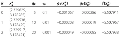
Table 5 Numerical results for Example 4.2 withx0= (1.0, 1.5)
k x∗k qk k g1(xk∗) g2(x∗k) f (xk∗)
0 (2.329625,
3.178285) 5 0.1 –0.001067 0.000286 –5.507911
1 (2.329538,
3.178429) 10 0.01 –0.000208 0.000019 –5.507967
2 (2.329517,
3.178421) 20 0.001 –0.000049 –0.000085 –5.507938
Letk= /,x= (., .),q= ,= .,η= .,σ = , = –, the results by Algo-rithm . are shown in Table .
With different starting pointsx= (., ),x= (, ), andx= (., .), numerical re-sults are given in Table , Table and Table , respectively. One can see that the numerical results in Tables - are similar. This means that Algorithm . does not completely de-pend on how to choose a starting point in this example. In [], the given solution for Example . is (., .) with objective function value –.. Numerical results are similar to the result of [] in this example.
For thejth iteration of the algorithm, we define a constraint errorejby
ej= m
i=
maxgi
x∗j , .
It is clear thatx∗j is-feasible to (P) whenej<.
Example .(Example . in [] and Example . in [])
minf(x) = x+ x+x+ x+ x,
s.t.g(x) =x+x– = ,
g(x) = –x+x+x+x= ,
g(x) = –x–x+x+x= ,
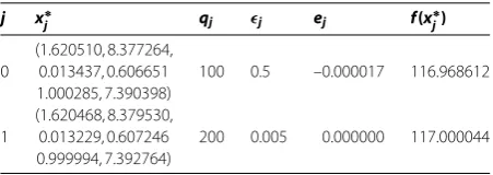
[image:10.595.179.414.299.375.2]Table 6 Numerical results for Example 4.3
j x∗j qj j ej f (x∗j)
0
(1.620510, 8.377264, 0.013437, 0.606651 1.000285, 7.390398)
100 0.5 –0.000017 116.968612
1
(1.620468, 8.379530, 0.013229, 0.607246 0.999994, 7.392764)
200 0.005 0.000000 117.000044
g(x) =x+ x+x– ≤, ≤x≤,
≤x≤, ≤x≤, ≤x≤, ≤x≤, ≤x≤.
Letk= /,x= (, , , , , ),q= ,= .,η= .,σ= ,= –, the results by Algorithm . are shown in Table .
It is clear from Table that the obtained approximately optimal solution is x∗ = (., ., ., ., ., .) with corresponding ob-jective function value .. In [], the obtained approximately optimal solution is x∗ = (., ., ., ., ., .) with correspond-ing objective function value .. In [], the given solution for Example . is (., ., ., ., ., .) with objective function value . whenk= /. Numerical results are better than the results of [] and [] in this example.
5 Concluding remarks
In this paper, we propose a method for smoothing the nonsmooth lower-order exact penalty function for inequality constrained optimization. We prove that the algorithm based on the smoothed penalty functions is convergent under mild conditions.
According to the numerical results given in Section , we can obtain an approximately optimal solution of the original problem [P] by Algorithm ..
Finally, we give some advices on how to choose parameter in the algorithm. Usually, the initial value ofqmay be , , , , or , andσ= , , or . The initial value ofmay be , ., . or ., andη= ., ., . or ..
Competing interests
The authors declare that they have no competing interests.
Authors’ contributions
Acknowledgements
The authors wish to thank the anonymous referees for their endeavors and valuable comments. This work is supported by National Natural Science Foundation of China (71371107 and 61373027) and Natural Science Foundation of Shandong Province (ZR2013AM013).
Received: 2 February 2016 Accepted: 8 July 2016
References
1. Zangwill, WI: Non-linear programming via penalty functions. Manag. Sci.13(5), 344-358 (1967) 2. Zangwill, I: A smoothing-out technique for min-max optimization. Math. Program.19(1), 61-77 (1980)
3. Ben-Tal, A, Teboulle, M: A smoothing technique for non-differentiable optimization problems. In: Lecture Notes in Mathematics, vol. 1405, pp. 1-11. Springer, Berlin (1989)
4. Pinar, M, Zenios, S: On smoothing exact penalty functions for convex constrained optimization. SIAM J. Optim.4, 486-511 (1994)
5. Liu, BZ: On smoothing exact penalty functions for nonlinear constrained optimization problems. J. Appl. Math. Comput.30, 259-270 (2009)
6. Lian, SJ: Smoothing approximation tol1exact penalty function for inequality constrained optimization. Appl. Math. Comput.219(6), 3113-3121 (2012)
7. Liu, BZ, Zhao, WL: A modified exact smooth penalty function for nonlinear constrained optimization. J. Inequal. Appl.
2012, 173 (2012)
8. Xu, XS, Meng, ZQ, Huang, LG, Shen, R: A second-order smooth penalty function algorithm for constrained optimization problems. Comput. Optim. Appl.55(1), 155-172 (2013)
9. Jiang, M, Shen, R, Xu, XS, Meng, ZQ: Second-order smoothing objective penalty function for constrained optimization problems. Numer. Funct. Anal. Optim.35(3), 294-309 (2014)
10. Binh, NT: Smoothing approximation tol1exact penalty function for constrained optimization problems. J. Appl. Math. Inform.33(3-4), 387-399 (2015)
11. Luo, ZQ, Pang, JS, Ralph, D: Mathematical Programs with Equilibrium Constraints. Cambridge University Press, Cambridge (1996)
12. Rubinov, AM, Yang, XQ, Bagirov, AM: Penalty functions with a small penalty parameter. Optim. Methods Softw.17(5), 931-964 (2002)
13. Huang, XX, Yang, XQ: Convergence analysis of a class of nonlinear penalization methods for constrained optimization via first-order necessary optimality conditions. J. Optim. Theory Appl.116(2), 311-332 (2003)
14. Wu, ZY, Bai, FS, Yang, XQ, Zhang, LS: An exact lower order penalty function and its smoothing in nonlinear programming. Optimization53(1), 51-68 (2004)
15. Meng, ZQ, Dang, CY, Yang, XQ: On the smoothing of the square-root exact penalty function for inequality constrained optimization. Comput. Optim. Appl.35, 375-398 (2006)
16. Lian, SJ: Smoothing approximation to the square-order exact penalty functions for constrained optimization. J. Appl. Math.2013, Article ID 568316 (2013)
17. He, ZH, Bai, FS: A smoothing approximation to the lower order exact penalty function. Oper. Res. Trans.14(2), 11-22 (2010)
18. Lian, SJ: On the smoothing of the lower order exact penalty function for inequality constrained optimization. Oper. Res. Trans.16(2), 51-64 (2012)
19. Bazaraa, MS, Sherali, HD, Shetty, CM: Nonlinear Programming: Theory and Algorithms, 2nd edn. Wiley, New York (1993)
20. Sun, XL, Li, D: Value-estimation function method for constrained global optimization. J. Optim. Theory Appl.102(2), 385-409 (1999)