Hybrid simultaneous algorithms for the split equality problem with applications

(1)

R E S E A R C H

Open Access

Hybrid simultaneous algorithms for the

split equality problem with applications

Chih-Sheng Chuang

1

_{and Wei-Shih Du}

2*

*_{Correspondence:}

[email protected]

2_{Department of Mathematics,}

National Kaohsiung Normal University, Kaohsiung, 82444, Taiwan

Full list of author information is available at the end of the article

Abstract

The split equality problem has board applications in many areas of applied mathematics. Many researchers studied this problem and proposed various

algorithms to solve it. From the literature we know that most algorithms for the split equality problems came from the idea of the projected Landweber algorithm proposed by Byrne and Moudafi (Working paper UAG, 2013), and few algorithms came from the idea of the alternating CQ-algorithm given by Moudafi (Nonlinear Anal. 79:117-121, 2013). Hence, it is important and necessary to give new algorithms from the idea of the alternating CQ-algorithm. In this paper, we first present a hybrid projected Landweber algorithm to study the split equality problem. Next, we propose a hybrid alternating CQ-algorithm to study the split equality problem. As applications, we consider the split feasibility problem and linear inverse problem. Finally, we give numerical results for the split feasibility problem to demonstrate the efficiency of the proposed algorithms.

MSC: 49J53; 49M37; 90C25

Keywords: split equality problem; split feasibility problem; split equality problem; linear inverse problem; simultaneous algorithm

1 Introduction

LetHbe a real Hilbert space with inner product·,·and norm · . We denote the strong convergence and weak convergence of{xn}n∈Ntox∈Hbyxn→xandxnx, respectively.

The symbolsNandRare used to denote the sets of positive integers and real numbers, respectively. For eachx∈H, there is a unique elementx¯∈Csuch thatx–x¯=min_y∈Cx–

y. In this study, we setPCx=x¯, andPCis called the metric projection fromHontoC. LetH andHbe two real Hilbert spaces. LetA:H→H andA∗:H→H be two

linear and bounded operators. ThenA∗is called the adjoint ofAifAz,w=z,A∗wfor all

z∈Handw∈H. It is known that the adjoint operator of a linear and bounded operator

on a Hilbert space always exists and is linear, bounded, and unique. Further, we know that A=A∗.

LetH,H, andHbe real Hilbert spaces. LetCandQbe nonempty closed convex

sub-sets ofH andH, respectively. LetA:H→HandB:H→Hbe linear and bounded

operators with adjoint operatorsA∗ andB∗, respectively. The following problem is the split equality problem, which was studied by Moudaﬁ [, ]:

(SEP) Findx¯∈Candy¯∈Qsuch thatAx¯=By¯.

(2)

Let:={(x,y)∈C×Q:Ax=By}be the solution set of problem (SEP). Further, we ob-served that (x,y) is a solution of the split equality problem if and only if

x=PC(x–ρA∗(Ax–By)),

y=PQ(y+ρB∗(Ax–By)),

for allρ>  andρ>  (for details, see []).

As mentioned by Moudaﬁ [], the interest of the split equality problem covers many situations, for instance, in decomposition methods for PDEs, game theory, and intensity modulated radiation therapy (IMRT). For details, see [, , ]. To solve problem (SEP), Moudaﬁ [] proposed the alternating CQ-algorithm:

(ACQA)

xn+:=PC(xn–ρnA∗(Axn–Byn)),

yn+:=PQ(yn+ρnB∗(Axn+–Byn)), n∈N,

whereH=RN,H=RM,PCis the metric projection mapping fromHontoC, andPQis

the metric projection mapping fromHontoQ,ε> ,Ais aJ×Nmatrix,Bis aJ×M

matrix,λAandλBare the spectral radii ofA∗AandB∗B, respectively, and{ρn}is a sequence

in (ε,min{_λ

A,



λB}–ε).

In , Byrne and Moudaﬁ [] presented a simultaneous algorithm, which was called the projected Landweber algorithm, to study the split equality problem

(PLA)

xn+:=PC(xn–ρnA∗(Axn–Byn)),

yn+:=PQ(yn+ρnB∗(Axn–Byn)), n∈N,

whereH=RN,H=RM,PCis the metric projection mapping fromHontoC, andPQis

the metric projection mapping fromHontoQ,ε> ,Ais aJ×Nmatrix,Bis aJ×M

matrix,λAandλBare the spectral radii ofA∗AandB∗B, respectively, and{ρn}is a sequence

in (ε,_λ 

A+λB).

Besides, we also observed that Chenet al.[] gave the following modiﬁcation of (ACQA) by using the Tikhonov regularization method and proved a convergence theorem under suitable conditions:

(TRA)

xn+:=PC(( –εnρn)xn–ρnA∗(Axn–Byn)),

yn+:=PQ(( –εnρn)yn+ρnB∗(Axn+–Byn)), n∈N,

where{εn}n∈Nis a sequence in (,∞). Besides, many researchers studied problem (SEP)

and gave various algorithms. For more details about the algorithms for the split equality problem, we refer to [, ] and related references.

(3)

numer-ical results for the split feasibility problem to demonstrate the eﬃciency of the proposed algorithms.

2 Main results

In the sequel, we need the following lemma, which is a crucial tool for our results.

Lemma .[] Let C be a nonempty closed convex subset of a real Hilbert space H,and let PCbe the metric projection from H onto C.Then:

(i) x–PCx,PCx–y ≥for allx∈Handy∈C;

(ii) x–PCx+PCx–y≤ x–yfor allx∈Handy∈C;

(iii) PCx–PCy≤ x–y,PCx–PCyfor allx,y∈H.

2.1 Hybrid projected Landweber algorithm

LetH,H, andH be real Hilbert spaces with inner product·,·Hi and norm · Hi, i= , , . For simplicity, we write·,·and · . LetCandQbe nonempty closed con-vex subsets ofH andH, respectively. LetA:H→H andB:H→H be linear and

bounded operators with adjoint operatorsA∗ andB∗, respectively. Chooseδ∈(, ). Let be the solution set of the split equality problem and suppose that=∅. Let{ρn}n∈Nbe

a sequence in (,∞).

Now we present a hybrid projected Landweber algorithm to study the split equality problem.

Algorithm . For givenxn∈H andyn∈H, ﬁnd the approximate solution by the

fol-lowing iterative process.

Step . Compute the next iterate(un,vn)as follows:

un=PC[xn–ρnA∗(Axn–Byn)], vn=PQ[yn+ρnB∗(Axn–Byn)],

whereρn> satisﬁes

ρ_nA∗(Axn–Byn) –A∗(Aun–Bvn)



+B∗(Axn–Byn) –B∗(Aun–Bvn)



≤δxn–un+δyn–vn,  <δ< . (.)

Step . Ifxn=unandyn=vn, then(xn,yn)is a solution of problem (SEP) and stop. Other-wise, go to Step .

Step . Compute the next iterate(xn+,yn+)as follows:

⎧ ⎪ ⎪ ⎪ ⎪ ⎪ ⎪ ⎨ ⎪ ⎪ ⎪ ⎪ ⎪ ⎪ ⎩

D(n,):=xn–un+ρn[A∗(Aun–Bvn) –A∗(Axn–Byn)], D(n,):=yn–vn–ρn[B∗(Aun–Bvn) –B∗(Axn–Byn)], αn:=xn

–un,D(n,)+yn–vn,D(n,) D(n,)+D(n,) , xn+=PC[xn–αnD(n,)],

yn+=PQ[yn–αnD(n,)].

(4)

Remark . If  <ρn≤ √

δ

√

(A₊_B₎, then (.) holds.

Proof Without loss of generality, we may assume that xn=un andyn=vn. We know

that

ρ_n·A∗(Axn–Byn) –A∗(Aun–Bvn)+B∗(Axn–Byn) –B∗(Aun–Bvn)

≤ρ_n·A∗+B∗·(Axn–Byn) – (Aun–Bvn)



≤ρ_n·A∗+B∗·A · xn–un+B · yn–vn 

≤ρ_n·A+B·A· xn–un+B· yn–vn

≤ρ_n·A+B·xn–un+yn–vn

≤· δ

(A₊_B₎ ·

A+B·xn–un+yn–vn

=δ·xn–un+yn–vn.

Therefore, the proof is completed.

Theorem . Let{ρn}n∈Nbe a sequence in(, /(A+B))such that(.)holds and

assume thatlim infn→∞ρn( –ρn(A+B)) > .Then,for the sequence{(xn,yn)}n∈Nin Algorithm.,there exists(x¯,y¯)∈such that xnx and yn¯ y as n¯ → ∞.

Proof Take anyn∈Nand letnbe ﬁxed. Take any (u¯,v¯)∈and let (u¯,v¯) be ﬁxed. Then ¯

u∈C,v¯∈Q, andAu¯=Bv¯. First, we set

εn,:=ρn[A∗(Aun–Bvn) –A∗(Axn–Byn)],

εn,:=ρn[B∗(Axn–Byn) –B∗(Aun–Bvn)].

Then

xn–un,D(n,)+yn–vn,D(n,)

=xn–un,xn–un+εn,+yn–vn,yn–vn+εn,

=xn–un+xn–un,εn,+yn–vn+yn–vn,εn,

=

xn–un

₊_xn_–_un_,_ε

n,+



xn–un



+

yn–vn

₊_yn_–_vn_,_ε

n,+



yn–vn



≥

xn–un

₊_xn_–_un_,_ε

n,+

 εn,



+

yn–vn

₊_y

n–vn,εn,+

 εn,



=

xn–un+εn,

₊

yn–vn+εn,



= D(n,)

₊

D(n,)

(5)

By (.) we know that

αn:=

xn–un,D(n,)+yn–vn,D(n,) D(n,)+D(n,) ≥



. (.)

Next, by Lemma . we know that

xn–αnD(n,)–xn++xn+–u¯≤ xn–αnD(n,)–u¯ (.)

and

yn–αnD(n,)–yn++yn+–v¯≤ yn–αnD(n,)–¯v. (.)

Hence, by (.),

xn–u¯–xn+–u¯

≥ xn–u¯–xn–αnD(n,)–u¯+xn+–xn+αnD(n,) ≥ xn–u¯–xn–αnD(n,)–u¯

=xn–u¯–xn–u¯–α_nD(n,)+ αnxn–u¯,D(n,)

= αnxn–u¯,D(n,)–αnD(n,). (.)

Similarly, we have

yn–v¯–yn+–v¯≥αnyn–v¯,D(n,)–αnD(n,). (.)

By (.) and (.) we get

xn+–u¯+yn+–v¯

≤ xn–u¯+yn–v¯– αnxn–u¯,D(n,)– αnyn–¯v,D(n,)

+α_nD(n,)+D(n,)

. (.)

Next, we know that

un–u¯,D(n,)+vn–v¯,D(n,)

=un–u¯,xn–un+ρn

A∗(Aun–Bvn) –A∗(Axn–Byn)

+vn–v¯,yn–vn–ρn

B∗(Aun–Bvn) –B∗(Axn–Byn)

=un–u¯,xn–un–ρnA∗(Axn–Byn)+un–u¯,ρnA∗(Aun–Bvn)

+vn–v¯,yn–vn+ρnB∗(Axn–Byn)–vn–v¯,ρnB∗(Aun–Bvn). (.)

By Lemma .,

(6)

and

vn–¯v,yn+ρnB∗(Axn–Byn) –vn≥. (.)

Besides, we also have

un–u¯,A∗(Aun–Bvn)–vn–¯v,B∗(Aun–Bvn)

=Aun–Au¯,Aun–Bvn–Bvn–Bv¯,Aun–Bvn

=Aun–Bvn–Au¯+Bv¯,Aun–Bvn

=Aun–Bvn,Aun–Bvn

=Aun–Bvn≥. (.)

So, by (.), (.), (.), and (.) we determine that

un–u¯,D(n,)+vn–v¯,D(n,) ≥, (.)

which implies that

xn–u¯,D(n,)+yn–v¯,D(n,) ≥ xn–un,D(n,)+yn–vn,D(n,). (.)

By (.), (.), and (.),

xn+–u¯+yn+–v¯

+α_nD(n,)+D(n,)

≤ xn–u¯+yn–v¯– αn

+α_nD(n,)+D(n,)

=xn–u¯+yn–v¯–αn

≤ xn–u¯+yn–v¯. (.)

So,{xn–u¯+yn–v¯}is a decreasing sequence, andlimn→∞xn–u¯+yn–v¯exists.

Further,{xn}n∈Nand{yn}n∈Nare bounded sequences, and

lim

n→∞xn–un,D(n,)+yn–vn,D(n,)= . (.)

Besides, we know that

=xn–un,xn–un+εn,+yn–vn,yn–vn+εn,

(7)

which implies that

xn–un+yn–vn

=xn–un,D(n,)+yn–vn,D(n,)–xn–un,εn,–yn–vn,εn,

≤ xn–un,D(n,)+yn–vn,D(n,)+xn–un · εn,+yn–vn · εn,

≤ xn–un,D(n,)+yn–vn,D(n,)+

 

xn–un+εn,+yn–vn+εn,

 +δ  ·

xn–un+yn–vn. (.)

Hence, by (.) we derive that

( –δ)xn–un+yn–vn≤xn–un,D(n,)+ yn–vn,D(n,). (.)

By (.) and (.) we know that

lim

n→∞xn–un=n→∞lim yn–vn= . (.)

By Lemma . again,

un–u¯ =PC

xn–ρnA∗(Axn–Byn)

–PC[u¯]



≤xn–ρnA∗(Axn–Byn) –u¯

≤ xn–u¯+ρ_nA· Axn–Byn– ρnAxn–Byn,Axn–Au¯. (.)

Similarly,

vn–v¯≤ yn–v¯+ρ_nB· Axn–Byn+ ρnAxn–Byn,Byn–Bv¯. (.)

By (.) and (.),

un–u¯+vn–v¯

≤ xn–u¯+yn–v¯+ρ_nA+B· Axn–Byn

– ρnAxn–Byn,Axn–Au¯+ ρnAxn–Byn,Byn–B¯v

=xn–u¯+yn–v¯–ρn

 –ρn

A+B· Axn–Byn. (.)

We also have

un–u¯+vn–v¯=un–xn+ un–xn,xn–u¯+xn–u¯

+vn–yn+ vn–yn,yn–¯v+yn–¯v. (.)

By (.), (.), and (.) we get

lim

(8)

Since{xn}n∈Nand{yn}n∈Nare bounded sequences, there exist subsequences{xnk}k∈Nand

{yn_k}k∈Nof{xn}n∈Nand{yn}n∈N, respectively, such thatxnkx¯andynky¯for somex¯∈H

andy¯∈H. Since{xn}∞n=is a sequence inC, we know thatx¯∈C. Also,y¯∈Q. Sincexnkx¯

andynky¯, it is easy to see thatAxnk Ax¯andBynk By¯by using the properties ofA

andB. Further,Axn_k–Byn_kAx¯–B¯y, and the lower semicontinuity of the squared norm implies

Ax¯–By¯≤lim inf

k→∞ Axnk–Bynk

₌ _lim

n→∞Axn–Byn

_{= .} _(.)

ThenAx¯=By¯and (x¯,y¯)∈.

Next, let{x_n_k}and{y_n_k}be other subsequences of{xn}n∈Nand{yn}n∈Nsuch thatx_n_kxˆ

andy_n_k yˆ, respectively. Following the same argument as before, we get that (xˆ,ˆy)∈. Besides, we have

xn–x¯+yn–y¯

=xn–xˆ+ˆx–x¯+ xn–xˆ,xˆ–x¯

+yn–ˆy+ˆy–y¯+ yn–ˆy,yˆ–y¯ (.)

and

xn–xˆ+yn–yˆ

=xn–x¯+ˆx–x¯+ xn–x¯,x¯–xˆ

+yn–¯y+ˆy–y¯+ yn–¯y,y¯–yˆ. (.)

Clearly,lim_n→∞xn–x¯₊_yn_–_y_¯_{exists, and}_lim

n→∞xn–xˆ+yn–yˆexists. Hence,

by (.) we get

lim

n→∞

= lim

k→∞x nk–x¯



+y_n_k–y¯

= lim

k→∞x nk–xˆ



+y_n_k–yˆ+ˆx–x¯+ˆy–y¯

+ lim

k→∞

x_n_k–xˆ,xˆ–x¯+  lim

k→∞

y_n_k–yˆ,yˆ–y¯

= lim

k→∞x nk–xˆ



+y_n_k–yˆ+ˆx–x¯+ˆy–y¯

= lim

n→∞

xn–xˆ+yn–ˆy

+ˆx–x¯₊_ˆ_y_–_¯_y_. _(.)

Similarly, by (.) we have

lim

n→∞

xn–xˆ+yn–ˆy

= lim

n→∞

+ˆx–x¯+ˆy–y¯. (.)

By (.) and (.) we know thatx¯=xˆandy¯=yˆ. Therefore,xnx¯andyny¯, and the

(9)

Remark . In Theorem ., if we choose{ρn}n∈N from (,√_(_Aδ₊_B₎], then we only

need to assume thatlim inf_n→∞ρn> . Proof Sinceρn∈(,√_(_Aδ₊_B₎], we have

ρn

A+B≤√·ρn·

A+B≤δ, ∀n∈N, (.)

which implies that

 –ρn

A+B≥ –δ> , ∀n∈N. (.)

Sincelim infn→∞ρn> , we may assume that there isκsuch thatρn≥κ>  for alln∈N.

Hence, we determine

ρn

 –ρn

A+B≥κ·( –δ) >κ, ∀n∈N. (.)

By (.) we get the conclusion of Remark ..

2.2 Hybrid alternating CQ-algorithm

In this subsection, we present a hybrid alternating CQ-algorithm to study the split equality problem.

Algorithm . For givenxn∈Handyn∈H, ﬁnd the approximate solution by the

Step . Compute the next iterate(un,vn)as follows:

un=PC[xn–ρnA∗(Axn–Byn)],

vn=PQ[yn+ρnB∗(Aun–Byn)],

ρ_nA∗(Axn–Byn) –A∗(Aun–Bvn)+B∗(Aun–Byn) –B∗(Aun–Bvn) ≤δxn–un+δyn–vn,  <δ< . (.)

Step . Ifxn=unandyn=vn, then(xn,yn)is a solution of problem (SEP) and stop.

Other-wise, go to Step .

⎧ ⎪ ⎪ ⎪ ⎪ ⎪ ⎪ ⎨ ⎪ ⎪ ⎪ ⎪ ⎪ ⎪ ⎩

D(n,):=xn–un+ρn[A∗(Aun–Bvn) –A∗(Axn–Byn)], D(n,):=yn–vn–ρn[B∗(Aun–Bvn) –B∗(Aun–Byn)], αn:=

xn–un,D(n,)+yn–vn,D(n,) D(n,)+D(n,) , xn+=PC[xn–αnD(n,)],

(10)

Remark . If  <ρn≤

√

δ

max{√·A_,√__·A_·|B₊_B_}, then (.) holds.

Proof Without loss of generality, we may assume thatxn=unandyn=vn. We have

ρ_n·A∗(Axn–Byn) –A∗(Aun–Bvn)



+B∗(Aun–Byn) –B∗(Aun–Bvn)



≤ρ_n·A∗·(Axn–Byn) – (Aun–Bvn)



+B· yn–vn

≤ρ_n·A∗·Axn–Aun+Byn–Bvn+B· yn–vn

≤ρ_n·A∗·Axn–Aun+ Byn–Bvn+B· yn–vn

≤ρ_n·A∗· xn–un+A· B+B· yn–vn

≤δxn–un+δyn–vn.

Therefore, the proof is completed.

Theorem . Let{ρn}n∈Nbe a sequence in(, /max{A,B})such that(.)holds and assume thatlim inf_n→∞ρn( –ρnA) > orlim infn→∞ρn( –ρnB) > .Then,for the sequence{(xn,yn)}n∈N in Algorithm.,there exists(x¯,y¯)∈such that xnx and¯ yn¯y as n→ ∞.

Proof Take anyn∈Nand letnbe ﬁxed. Take any (u¯,v¯)∈and let (u¯,v¯) be ﬁxed. Then ¯

u∈C,v¯∈Q, andAu¯=Bv¯. First, we set

εn,:=ρn[A∗(Aun–Bvn) –A∗(Axn–Byn)], εn,:=ρn[B∗(Aun–Byn) –B∗(Aun–Bvn)].

Then

xn–un,D(n,)+yn–vn,D(n,) ≥

 D(n,)

₊

D(n,)

_. _(.)

By (.) we have that

αn:=

xn–un,D(n,)+yn–vn,D(n,) D(n,)+D(n,) ≥



. (.)

Next, by Lemma . we have

xn–αnD(n,)–xn++xn+–u¯≤ xn–αnD(n,)–u¯ (.)

and

yn–αnD(n,)–yn++yn+–v¯≤ yn–αnD(n,)–¯v. (.)

Hence, by (.),

(11)

Also, by (.),

yn–v¯–yn+–v¯≥αnyn–v¯,D(n,)–αnD(n,). (.)

By (.) and (.) we get

xn+–u¯+yn+–v¯

+α_nD(n,)+D(n,)

. (.)

Next, we have

un–u¯,D(n,)+vn–v¯,D(n,)

=un–u¯,xn–un+ρn

A∗(Aun–Bvn) –A∗(Axn–Byn)

+vn–v¯,yn–vn–ρn

B∗(Aun–Bvn) –B∗(Aun–Byn)

=un–u¯,xn–un–ρnA∗(Axn–Byn)+un–u¯,ρnA∗(Aun–Bvn)

+vn–v¯,yn–vn+ρnB∗(Aun–Byn)–vn–v¯,ρnB∗(Aun–Bvn). (.)

By Lemma .,

un–u¯,xn–ρnA∗(Axn–Byn) –un≥ (.)

and

vn–¯v,yn+ρnB∗(Aun–Byn) –vn≥. (.)

Besides, we also have

un–u¯,A∗(Aun–Bvn)–vn–¯v,B∗(Aun–Bvn)=Aun–Bvn≥. (.)

So, by (.), (.), (.), and (.) we determine that

un–u¯,D(n,)+vn–v¯,D(n,) ≥, (.)

which implies that

xn–u¯,D(n,)+yn–v¯,D(n,) ≥ xn–un,D(n,)+yn–vn,D(n,). (.)

By (.), (.), and (.),

xn+–u¯+yn+–v¯

+α_nD(n,)+D(n,)

(12)

≤ xn–u¯+yn–v¯– αn

+α_nD(n,)+D(n,)

=xn–u¯+yn–v¯–αn

≤ xn–u¯+yn–v¯. (.)

So,{xn–u¯₊_yn_–_¯_v_}_{is a decreasing sequence,}_lim

n→∞xn–u¯+yn–v¯exists,

{xn}n∈Nand{yn}n∈Nare bounded sequences, and

lim

n→∞xn–un,D(n,)+yn–vn,D(n,)= . (.)

Besides, we have

=xn–un+xn–un,εn,+yn–vn+yn–vn,εn,, (.)

which implies that

xn–un+yn–vn

 +δ  ·

xn–un+yn–vn. (.)

Hence, by (.) we derive that

( –δ)xn–un+yn–vn≤xn–un,D(n,)+ yn–vn,D(n,). (.)

By (.) and (.) we get that

lim

n→∞xn–un=n→∞lim yn–vn= . (.)

By Lemma . again,

un–u¯ =PCxn–ρnA∗(Axn–Byn)–PC[u¯] ≤xn–ρnA∗(Axn–Byn) –u¯

≤ xn–u¯+ρ_nA· Axn–Byn

– ρnAxn–Byn,Axn–Au¯

=xn–u¯–ρn·

 –ρnA

· Axn–Byn

– ρnAxn–Byn,Byn–Au¯. (.)

Similarly,

(13)

≤ yn–v¯+ρ_nB· Aun–Byn

+ ρnAun–Byn,Byn–Bv¯

=yn–v¯–ρn

 –ρnB

· Aun–Byn

+ ρnAun–Byn,Aun–Bv¯. (.)

We also have

Axn–Byn,Byn–Au¯=Axn–Au¯–Axn–Byn–Byn–Au¯ (.)

and

Aun–Byn,Aun–B¯v=Aun–Bv¯+Aun–Byn–Byn–Bv¯. (.)

By (.), (.), (.), and (.),

un–u¯+vn–v¯

≤ xn–u¯+yn–v¯–ρn

 –ρnA

· Axn–Byn

–ρn

 –ρnB

· Aun–Byn+ρn

Aun–Au¯–Axn–Au¯

≤ xn–u¯+yn–v¯–ρn

 –ρnA

· Axn–Byn

–ρn

 –ρnB

· Aun–Byn

+ρn· A · un–xn ·

Aun–Au¯+Axn–Au¯. (.)

We also have

un–u¯+vn–v¯=un–xn+ un–xn,xn–u¯+xn–u¯

+vn–yn+ vn–yn,yn–¯v+yn–¯v. (.)

Case :lim inf_n→∞ρn( –ρnA) > .

By (.), (.), and (.) we get

lim

n→∞Axn–Byn= . (.)

Case : Suppose thatlim infn→∞ρn( –ρnB) > .

By (.), (.), and (.) we get

lim

n→∞Aun–Byn= . (.)

By (.) and (.) we determine

lim

n→∞Axn–Byn= . (.)

Next, following the same argument as the ﬁnal proof of Theorem ., we get the

(14)

Remark . Suppose that{ρn}n∈Nsatisfy the following inequality:

 <κ≤ρn≤

δ

max{√· A_,_· _A· _B₊_B_,_B}.

Then{ρn}n∈Nsatisfy the conditions in Remark . and Theorem ..

3 Applications of the split equality problem

3.1 The split feasibility problem

LetHandHbe real Hilbert spaces. LetCandQbe nonempty closed convex subsets of

H andH, respectively. LetA:H→Hbe a linear and bounded operator with adjoint

operatorA∗. The following problem is the split feasibility problem in Hilbert spaces, which was ﬁrst introduced by Censor and Elfving []:

(SFP) Findx¯∈Hsuch thatx¯∈CandAx¯∈Q.

Here, let:={x∈C:Ax∈Q}be the solution set of problem (SFP). It is worth noting

that this problem is a particular case of the split equality problem whenH=HandBis

the identity mapping onH. For additional details, one can refer to [, –] and related

literature.

By Algorithm ., we get the following algorithm to study problem (SFP).

Algorithm . For givenxn∈H andyn∈H, ﬁnd the approximate solution by the

Step . Forn∈N, letunandvnbe deﬁned by

un=PC[xn–ρnA∗(Axn–yn)], vn=PQ[yn+ρn(Aun–yn)],

ρ_nA∗(Axn–yn) –A∗(Aun–vn)+(Aun–yn) –B∗(Aun–vn)

≤δxn–un+δyn–vn,  <δ< . (.)

Step . Ifxn=unandyn=vn, then(xn,yn)is a solution of problem (SFP) and stop. Other-wise, go to Step .

⎧ ⎪ ⎪ ⎪ ⎪ ⎪ ⎪ ⎨ ⎪ ⎪ ⎪ ⎪ ⎪ ⎪ ⎩

D(n,):=xn–un+ρn[A∗(Aun–vn) –A∗(Axn–yn)], D(n,):=yn–vn–ρn[(Aun–vn) – (Aun–yn)], αn:=xn

–un,D(n,)+yn–vn,D(n,) D(n,)+D(n,) , xn+=PC[xn–αnD(n,)],

(15)

We get the following convergence theorem for the split feasibility problem by using The-orem ..

Theorem . Let Hand Hbe real Hilbert spaces.Let C and Q be nonempty closed

con-vex subsets of Hand H,respectively.Let A:H→Hbe a linear and bounded operator

with adjoint operator A∗.Chooseδ∈(, ).Letbe the solution set of the split feasibility

problem and suppose that=∅.Let{ρn}n∈N be a sequence in(, /max{A, })such that(.)hold and assume thatlim inf_n→∞ρn( –ρnA) > orlim infn→∞ρn( –ρn) > s. Then,for the sequence{(xn,yn)}n∈Nin Algorithm.,there existsx¯∈such that xnx¯

as n→ ∞.

3.2 Linear inverse problem

In this subsection, we study an inverse problem by our algorithms and convergence the-orems. LetHandHbe real Hilbert spaces. LetCbe a nonempty closed convex subset

ofH, andA:H→Hbe a linear and bounded operator with adjoint operatorA∗. Given

b∈H. Then we consider the following inverse problem in this section:

(IV) Findx¯∈Csuch thatAx¯=b.

This is a particular case of the split equality problem ifH=H,Q={b}, andB(x) =x

for allx∈H. Next, take any (x,y)∈H×Hwithy=b. Then, by Algorithm . we get

the following algorithm to study problem (IV).

Algorithm . For givenxn∈H, ﬁnd the approximate solution by the following iterative

process.

Step . Compute the next iterateunas follows:

un=PC

xn–ρnA∗(Axn–b)

,

ρ_n·A∗(Axn) –A∗(Aun)≤δxn–un,  <δ< . (.)

Step . Ifxn=un, thenxnis a solution of problem (IV) and stop. Otherwise, go to Step . Step . Compute the next iteratexn+as follows:

⎧ ⎪ ⎨ ⎪ ⎩

Dn:=xn–un+ρn[A∗(Aun) –A∗(Axn)], αn:=xn_D–u_nn,Dn,

xn+=PC[xn–αnDn].

Next, updaten:=n+ and go to Step .

We get the following convergence theorem for the linear inverse problem by using The-orem ..

Theorem . Let Hand H be real Hilbert spaces.Let C be a nonempty closed convex

subset of H,and A:H→Hbe a linear and bounded operator with adjoint operator A∗.

(16)

Let {ρn}n∈N be a sequence in (, /max{A, })such that (.)holds and assume that

lim inf_n→∞ρn( –ρnA) > orlim infn→∞ρn( –ρn) > .Then,for the sequence{xn}n∈N in Algorithm.,there existsx¯∈such that xnx as n¯ → ∞.

Remark . By Algorithm . and Theorem ., we can get the related algorithms and convergence theorems for the split feasibility problem and the inverse problems.

4 Numerical results

All codes were written in R language (version .. (--), the R Foundation for Statistical Computing Platform: x--w-mingw/x).

Example . LetH=H=H=R,C:={x∈R:x ≤},Q:={x= (u,v)∈R: (u–

)_{+ (}_v_{– )}_≤__}_,

A:=

 

 

, B:=

 

 

.

Then problem (SEP) has a unique solution (x¯,y¯)∈R×R, wherex¯:= (x¯,x¯),y¯:= (y¯,y¯).

Indeed,x¯= .,x¯= .,y¯= ,y¯= . Letε>  and the algorithm stop ifxn–x¯+yn– ¯

y<ε.

In Table , settingε= –,x= (, )T,y= (, )T, andρn= . for alln∈N, we get

the numerical results.

In Table , settingε= –_,_x

= (, )T,y= (, )T, andρn= . for alln∈N, we get the

numerical results.

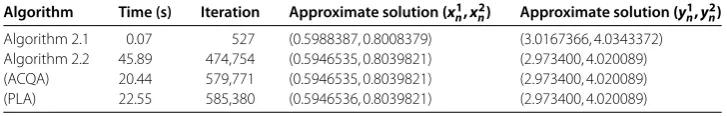
In Table , settingε= ×–_,_x

[image:16.595.116.480.490.547.2]

= (–, –)T,y= (–, )T, andρn= . for all n∈N, we get the numerical results.

Table 1 ε= 10–1,x1= (10, 10)T,y1= (1, 1)T,ρn= 0.01

Algorithm Time (s) Iteration Approximate solution(x1

[image:16.595.116.481.583.639.2]

n, x2n) Approximate solution(yn1, y2n) Algorithm 2.1 0.01 196 (0.6114674, 0.7912309) (3.0850778, 3.9920504) Algorithm 2.2 0.00 122 (0.5970952, 0.8020906) (3.0421971, 4.0866474) (ACQA) 1.94 58,324 (0.6132467, 0.7898914) (3.0670840, 3.9505550) (PLA) 2.57 78,654 (0.6132467, 0.7898914) (3.0670840, 3.9505550)

Table 2 ε= 10–1,x1= (5, 5)T,y1= (1, 1)T,ρn= 0.01

n, x2n) Approximate solution(yn1, y2n) Algorithm 2.1 0.82 11,168 (0.6132467, 0.7898915) (3.067084, 3.950555)

Algorithm 2.2 0.02 205 (0.6077392, 0.7940725) (3.0847143, 4.0304899) (ACQA) 1.94 58,324 (0.6132467, 0.7898914) (3.067084, 3.950555) (PLA) 2.28 71,521 (0.6132467, 0.7898915) (3.067084, 3.950555)

Table 3 ε= 4×10–2,x1= (12, –50)T,y1= (–40, 20)T,ρn= 0.01

[image:16.595.116.480.675.733.2]

(17)

Competing interests

The authors declare that they have no competing interests.

Authors’ contributions

Both authors contributed equally and signiﬁcantly in writing this paper. Both authors read and approved the ﬁnal manuscript.

Author details

1_{Department of Applied Mathematics, National Chiayi University, Chiayi, Taiwan.}2_{Department of Mathematics, National}

Kaohsiung Normal University, Kaohsiung, 82444, Taiwan.

Acknowledgements

Prof. Wei-Shih Du was supported by Grant No. MOST 104-2115-M-017-002 of the Ministry of Science and Technology of the Republic of China.

Received: 10 May 2016 Accepted: 28 July 2016

References

1. Byrne, C, Moudaﬁ, A: Extensions of the CQ algorithms for the split feasibility and split equality problems. Working paper UAG (2013)

2. Moudafi, A: A relaxed alternating CQ-algorithm for convex feasibility problems. Nonlinear Anal.79, 117-121 (2013) 3. Moudafi, A: Alternating CQ-algorithms for convex feasibility and split fixed-point problems. J. Nonlinear Convex Anal.

15, 809-818 (2014)

4. Dong, QL, He, S: Solving the split equality problem without prior knowledge of operator norms. Optimization64, 1887-1906 (2015)

5. Attouch, H, Bolte, J, Redont, P, Soubeyran, A: Alternating proximal algorithms for weakly coupled minimization problems. Applications to dynamical games and PDEs. J. Convex Anal.15, 485-506 (2008)

6. Censor, Y, Bortfeld, T, Martin, B, Troﬁmov, A: A uniﬁed approach for inversion problems in intensity-modulated radiation therapy. Phys. Med. Biol.51, 2353-2365 (2006)

7. Chen, R, Li, J, Ren, Y: Regularization method for the approximate split equality problem in inﬁnite-dimensional Hilbert spaces. Abstr. Appl. Anal.2013, Article ID 813635 (2013)

8. Dong, QL, He, S: Modiﬁed projection algorithms for solving the split equality problems. Sci. World J.2014, Article ID 328787 (2014)

9. Vuong, PT, Strodiot, JJ, Nguyen, VH: A gradient projection method for solving split equality and split feasibility problems in Hilbert spaces. Optimization64, 2321-2341 (2015)

10. Takahashi, W: Introduction to Nonlinear and Convex Analysis. Yokohama Publishers, Yokohama (2009)

11. Censor, Y, Elfving, T: A multiprojection algorithm using Bregman projection in a product space. Numer. Algorithms8, 221-239 (1994)

12. Byrne, C: Iterative oblique projection onto convex sets and the split feasibility problem. Inverse Probl.18, 441-453 (2002)

13. Byrne, C: A uniﬁed treatment of some iterative algorithms in signal processing and image reconstruction. Inverse Probl.20, 103-120 (2004)

14. Dang, Y, Gao, Y: The strong convergence of a KM-CQ-like algorithm for a split feasibility problem. Inverse Probl.27, 015007 (2011)

15. López, G, Martín-Márquez, V, Xu, HK: Iterative algorithms for the multiple-sets split feasibility problem. In: Censor, Y, Jiang, M, Wang, G (eds.) Biomedical Mathematics: Promising Directions in Imaging, Therapy Planning and Inverse Problems, pp. 243-279. Medical Physics Publishing, Madison (2010)

16. Masad, E, Reich, S: A note on the multiple-set split convex feasibility problem in Hilbert space. J. Nonlinear Convex Anal.8, 367-371 (2008)

17. Qu, B, Xiu, N: A note on the CQ algorithm for the split feasibility problem. Inverse Probl.21, 1655-1665 (2005) 18. Stark, H: Image Recovery: Theory and Applications. Academic Press, San Diego (1987)

19. Wang, F, Xu, HK: Approximating curve and strong convergence of the CQ algorithm for the split feasibility problem. J. Inequal. Appl.2010, Article ID 102085 (2010)

20. Xu, HK: A variable Krasnosel’skii-Mann algorithm and the multiple-set split feasibility problem. Inverse Probl.22, 2021-2034 (2006)

21. Xu, HK: Iterative methods for the split feasibility problem in inﬁnite-dimensional Hilbert spaces. Inverse Probl.26, 105018 (2010)

22. Yang, Q: The relaxed CQ algorithm for solving the split feasibility problem. Inverse Probl.20, 1261-1266 (2004) 23. Yang, Q: On variable-step relaxed projection algorithm for variational inequalities. J. Math. Anal. Appl.302, 166-179

(2005)