On Mars Thermosphere, Ionosphere and Exosphere: 3D Computational Study of Suprathermal Particles

(1)

On Mars thermosphere, ionosphere and exosphere:

3D computational study of suprathermal particles

by

Arnaud Valeille

A dissertation submitted in partial fulfillment of the requirements for the degrees of

Doctor of Philosophy

(Atmospheric and Space Science and Scientific Computing) in the University of Michigan

2009

Doctoral Committee:

Research Professor Michael R. Combi, Chair Research Professor Stephen W. Bougher Professor Edward W. Larsen

(2)

“The time will come when diligent research over long periods will bring to light things which now lie hidden. A single lifetime, even though entirely devoted to the sky, would not be enough for the investigation of so vast a subject... And so this knowledge will be unfolded only through long successive ages. There will come a time when our descendents will be amazed that we did not know things that are so plain to them… Many discoveries are reserved for the ages still to come, when the memory of us will have been effaced. Our universe is a sorry little affair unless it has in it something for every age to investigate… Nature does not reveal her mysteries once and for all.”

(3)

(4)

A mes parents, Marie-Louise et Georges

ii

(5)

iii

Acknowledgements

First and foremost, I would like to thank my dissertation committee chair and academic advisor, Prof. Mike Combi. His continuous guidance, support, encouragement have made this work possible. I am grateful to him for giving me the intellectual freedom and challenge to follow two different Master programs at the same time in the Atmospheric and Space Science department (AOSS), College of Engineering and in the Mathematics department, College of Literature Science and Art (LSA), both at the University of Michigan. These additional interdisciplinary classes were highly beneficial and allowed me to follow this joint PhD program in both Space Science and Scientific Computing.

I would like to thank my dissertation committee, Prof. Mike Combi, Prof. Steve Bougher, Prof. Andy Nagy and Prof. Edward Larsen. Their careful reading, expert suggestions and valuable comments have strongly improved this thesis.

I am very thankful to Prof. Steve Bougher for sharing his wisdom with me, for his very detailed reviews and pertinent comments. I believe that we had a very rich collaboration in the three and half years I spent in the department and I learned a lot from him.

I would like to express my admiration for Prof. Andy Nagy. He has more than forty years of experience in both theoretical and experimental studies of planetary upper atmospheres and worked as principal and co-investigator of a variety of instruments flown on pioneering missions to space. I feel extremely lucky to have worked with him. He has permitted an international exchange with my French school Supaero and allows me to be part of today’s one of the best Space Science program in the world.

(6)

used for simulations around comets. Valeriy helped me substantially on using and modifying his code and on its adaptation to Mars.

I was delighted to meet the scientists from whom Space Science benefits so much, and I would like to thank them for their inspiring discussions. These chances came from the many opportunities I had to attend scientific conferences in different part of North America, including: Spring AGU 2007 (Acapulco, Mexico), DPS 2007 (Orlando, FL, USA), Fall AGU 2007 (San Francisco, CA, USA), COSPAR 2008 (Montreal, Canada), DPS 2008 (Ithaca, NY, USA) and Fall AGU 2008 (San Francisco, CA, USA).

This thesis is mostly built on four papers that benefited from excellent reviews of seven reviewers specialized in the field. I would like to thank them for their assistance in evaluating these papers.

For funding this work, I gratefully acknowledge the National Aeronautics and Space Administration (NASA). Support for this work comes from the NASA Mars Fundamental Research grant NNG05GL80G and the Mars Data Analysis Program grant NNX07AO84G. Computations were performed on the massively parallel Columbia computer at the High-End Computing (HEC) Program's NASA Advanced Supercomputing (NAS) Facility.

Finally, I would like to thank the French elite Classes préparatoires (equivalent of first years of undergraduate) education system for its cold scientific rigor and the US graduate education system for its supportive research freedom. I feel extremely lucky having both experiences.

iv

(7)

Foreword

The meaning of life is deeply mixed with the scientific and philosophical conceptions of survival and happiness. At the end of the 20th century, based upon insight gleaned from the gene-centered view of evolution, biologists George C. Williams, Richard Dawkins, David Haig, among others, conclude that if there is a primary function to life, it is the replication of DNA and the survival of one's genes. Attempts to find meaning in subjective sensory experience may involve a focus on immediate experience and gratification, as in various forms of hedonism or carpe diem philosophies, or in long-term efforts at the creation of an aesthetically pleasing life, as with Epicureanism. If the purpose of life involves these two concepts of seeking happiness and being useful to the next generation, then the fundamental human essence, feeling and motivation, that is the hunger for knowledge, could be seen as the main purpose of its existence. Therefore, driven by its insatiable curiosity, mankind is invariably confronted to the metaphysical questions: ‘What is the origin of life?’ and ‘How the universe was created?’.

v

(8)

vi

List of Figures

1.1 Planets and dwarf planets of the Solar System ...2

1.2 View of Mars from Hubble Space Telescope on June 26, 2001 ...3

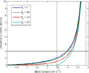
2.1 Altitude maximum reached by non-escaping particles ...15

2.2 Family of elliptical satellite orbits ...16

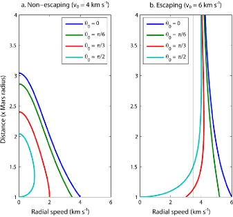
2.3 Radial component of the velocity for non-escaping (a) and escaping (b) particles for various initial pitch angle θ0. ...17

2.4 Time of flight in a 3-Martian-radius domain of study for particles with initial speed v0 up to 6.0 km s-1...19

2.5 Angular displacement (a) and angular deviation (b) due to an additional perpendicular push added to the initial velocity of the particle ...20

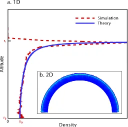
2.6 Density profile for radial non-escaping particles computed by 1D (a) and 2D (b) spherical simulations ...24

2.7 Density profile of an isotropic injection of non-escaping particles at the critical level r0 ...26

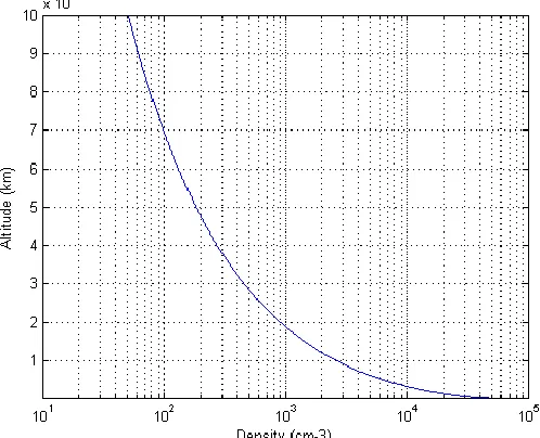
2.8 Density profile of an isotropic injection of escaping particles at the critical level r0 ..27

2.9 Density profiles of a thermal injection of particles at a critical level r0 ...29

3.1 Upper thermospheric fit of the neutrals (a) and ions (b) measurements made by Viking 1 & 2 descent missions in 1976 (extended to 300 km) [Source: Hanson et al. 1977] ...31

3.2 The distribution of O2+ ions with SZA (red line) assumed in the study of Chaufray et al. [2007] (the black lines are the functions used between 0-60°, 60-120°, 120-180° SZA, respectively). ...33

3.3 Validation of the code using 1D thermospheric inputs ...39

3.4 Section of the 3D tetrahedral mesh ...41

3.5 Density profiles and cold/hot ratios for different definitions of hot oxygen between 100 and 100,000 km altitude (a) and between 100 and 1000 km altitude (b) ...45

viii

(11)

3.6 Statistically averaged elastic (a) and differential (b) cross sections of oxygen atoms, as a function of the relative energy (a and b) and of the scattering angle (b) ...48 3.7 Maps of Mars global topography ...49 3.8 Illustration of the solar wind interaction on Mars ...52 3.9 Production rate as a function of SZA (along east Equatorial cut) and altitude in the upper thermosphere region (from 135 to 200 km altitude) at fixed orbital position of equinox for solar high conditions (EH case). ...54

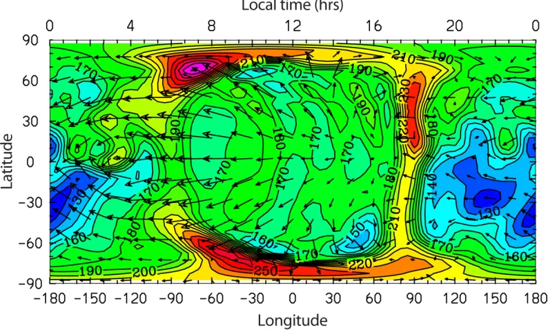
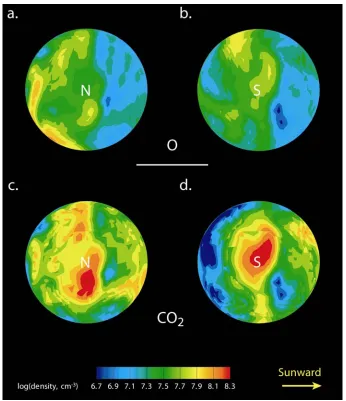
4.1 Neutral temperature at an altitude of 190 km. ...56 4.2 O density maps at the North (a) and South (b) hemispheres; CO2 density maps at the

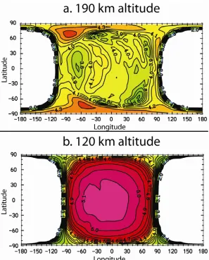
North (c) and South (d) hemispheres at an altitude of 190 km ...59 4.3 Surface map of O2+ ion log density (in cm-3) at altitudes of 190 km (a) and 120 km

(b) ...61 4.4 Maps of the oxygen mixing ratio, XO = O/(O+CO2), at the North (a) and South (b)

hemispheres at an altitude of 190 km, above which O becomes the main neutral

constituent of the Martian upper thermosphere on the average ...62 4.5 Oxygen mixing ratio, XO = O/(O+CO2), along a study path at the Equator from noon

(0° SZA) to midnight (180° SZA) through dusk in the region where the transition occurs

(130-330 km altitudes) ...63 4.6 Maps of the exobase criterion at the North (a) and South (b) hemispheres at an

altitude of 170 km ...66 4.7 Upward (red arrows up) and Downward (blue arrows down) hemispheric fluxes of hot oxygen atoms as functions of SZA for Equinox, Low solar activity, Equatorial east (ELE) conditions in the vicinity of the exobase (190 km altitude) ...68 4.8 Escape fluxes of hot oxygen atoms as functions of SZA for Equinox, High solar activity along the south Polar cut (EHP, orange dashed-dotted-dotted line) and the east Equatorial (EHE, dashed green line) at 10 Martian radii ...71 4.9 Flux of escaping hot oxygen atoms as functions of longitude and latitude at an

altitude surface of 2 Martian radii (~7000 km) in the frame associated with the Sun ...73 4.10 Flux of escaping hot oxygen atoms as functions of longitude and latitude at an altitude surface of 2 Martian radii (~7000 km) in the frame associated with Mars without winds (a) and with winds (b), and in the frame associated with the Sun (c) ...75 4.11 2D plot of the hot oxygen density and temperature profiles for Equinox, Low solar activity, Equatorial (ELE) conditions versus SZA (from noon to midnight through dawn) and the altitude (from 135 to 7000 km) ...76 4.12 Total oxygen density profile (purple solid line) as function of altitude (from 200 to 1000 km) at 60° SZA for Equinox, Low solar activity, south Equatorial east (ELE)

conditions ...77 4.13 Three-dimensional representation of the Martian hot corona. ...78 ix

(12)

4.14 O+ ionization rate (in s-1) in the equatorial section ...81

5.1 Neutral temperature in the vicinity of Mars exobase for low (a) and high (b) solar activity for modern conditions ...84 5.2 Average exospheric temperature function of the F10.7 cm index at Mars ...85 5.3 Oxygen mixing ratio in the winter hemisphere and neutral temperature in the vicinity of Mars exobase for the two most extreme cases for modern conditions ...86 5.4 Atomic oxygen in the vicinity of Mars exobase for low (a) and high (b) solar activity for modern conditions ...87 5.5 Surface map of O2+ ion log density (in cm-3) at altitudes of 190 km (a and b) and 120

km (c and d) for low (a and c) and high (b and d) solar activity for modern conditions ...90 5.6 Density profiles (a and c) and escape fluxes at 3 Martian radii (b and d) of oxygen atoms at Equinox for solar Low (EL, a and b) and High (EH, c and d) conditions ...93 5.7 Hot oxygen density altitude profiles function of SZA and solar activity between 200 and 7000 km (~3 planet radii) altitude, along the Equator east ...94 5.8 Comparative histogram of the hot atomic oxygen escape rates due to O2+ DR with

other models of the last ten years for low (blue) and high (red) solar activity ...96 5.9 Density profiles (a, c and e) and escape fluxes at 3 Martian radii (b, d and f) of

oxygen atoms for solar low activity at Aphelion (AL, a and b), Equinox (EL, b and c) and Perihelion (PL, e and f) ...97 5.10 Escape fluxes of hot oxygen atoms along the south Polar cut as a function of SZA for PHP (solid red line), EHP (dashed-dotted-dotted orange line), ELP (dashed-dotted light blue line) and ALP (dashed dark blue line) conditions at 10 Martian radii ...99 5.11 Density profiles (a and c) and escape fluxes at 3 Martian radii (b and d) of oxygen atoms for the two most extreme cases for modern conditions, Aphelion solar Low (AL, a and b) and Perihelion solar High (PH, c and d) ...101 5.12 Trends of the measured solar activity at Earth (1 AU) ...103

6.1 Profile of the neutral temperature in the Martian upper thermosphere (120 to 300 km altitude) at the equatorial noon (0° SZA) for epoch 1, 2 and 3 (blue, green and red lines,

respectively) for solar low conditions ...109 6.2 Surface maps of the neutral temperature for epoch 1, 2, 3 (a, b, c, respectively) for solar low conditions at 190 km altitude ...111 6.3 Oxygen mixing ratio in the winter hemisphere (a, c and e) and neutral temperature in the vicinity of Mars exobase (b, d and f) at epoch 1, 2 and 3 ...113 6.4 Density profiles of the two main neutral constituents of the Martian upper

thermosphere (120 to 280 km altitude), CO2 (a) and O (b), at the equatorial noon, 0°

SZA, and midnight, 180° SZA, (solid and dashed lines, respectively) for epoch 1, 2, a

(blue, green and red lines, respectively) for solar low conditions ...114 nd 3

x

(13)

xi

6.5 O2+ density profile in the Martian upper thermosphere (100 to 200 km altitude) at the

equatorial noon (0° SZA) for epoch 1, 2 and 3 (blue, green and red lines, respectively) for

solar low conditions ...118 6.6 Density profiles (a, c and e) and escape fluxes at 3 Martian radii (b, d and f) of

oxygen atoms at epoch 1, 2 and 3 ...121 6.7 . Escape fluxes of hot oxygen atoms along the equatorial cut from 0 to 180° SZA

(noon to midnight, through dawn) for Equinox at 10 Martian radii for epoch 1, 2 and 3 (blue, green and red lines, respectively) for both solar minimum (solid lines) and

maximum (dashed lines) conditions ...122 6.8 Hot oxygen density altitude profiles as a function of SZA between 200 and 7000 km (~2 planet radii) altitude, along the east Equator for solar low conditions ...123 6.9 Linear regression of neutral O escape rate due to DR (red lines), due to sputtering (black line) and O+ ions production rate (blue lines) versus EUV flux of epochs 1, 2 and 3 for solar minimum (solid lines) and maximum (dashed-dotted lines) conditions ...130 6.10 Cumulative water loss due to sputtering, ion loss (blue lines) and DR (red lines) for solar minimum (solid lines) and maximum (dashed-dotted lines) conditions ...132

7.1 The two most important groups of oxygen escape mechanisms on Mars: DR of thermospheric O2+ ions and processes due to ionospheric O+ pickup ions precipitation

(more specifically: ions, sputtering and ENA escape processes) ...134 7.2 Spatial distributions of the precipitating flux at an altitude of 300 km above the

Martian surface ...137 7.3 Hot oxygen density due to the sputtering for (a) low and (b) high solar conditions in the equatorial plane (the grey scale is in log10 of cm-3) ...139

7.4 Density profile of escaping oxygen atoms due to sputtering (a) and due to O2+ DR (b)

for the EL case ...140 7.5 Density profile of escaping carbon atoms due to CO photodissociation for the EL case. ...144

(14)

List of Tables

2.1 Escape speeds at the planets of the solar system ...12 3.1 Illustration of the necessity of combining hydrodynamic and kinetic models to

describe rigorously both transitional and collisionless regions [adapted from Valeille et al. 2009a] ...42 3.2 Number of iterations reached by a simulation, function of Vthreshold ...46

4.1 Ionization of cold and hot atomic oxygen by the three main ionization contributions; PI, CE and EI ...80 5.1 Impact of season and solar cycle on thermospheric/ionospheric parameters ...89 5.2 Comparative study of the Martian hot atomic oxygen escape rates due to O2+ DR with

other exospheric models of the last ten years with their respective thermospheric inputs and respective dimension (1D, 2D, 3D) of the simulations ...95 5.3 Impact of season and solar cycle on the escape rate of suprathermal oxygen atoms ..98 6.1 Scale heights (in km) of the main neutral (CO2 and O) and ion (O2+) constituents of

the Martian upper thermosphere at noon and midnight for epoch 1, 2 and 3 for solar minimum conditions ...115 6.2 Altitude (km), above which O becomes the main neutral constituent of the Martian upper thermosphere, for epoch 1, 2 and 3 for both solar minimum and maximum conditions (dayside and nightside values are presented along with the average value, rounded to nearest 5 km) ...116 6.3 Average exobase altitude (km) function of different Martian epochs for both solar minimum and maximum conditions, rounded to nearest 5 km ...119 6.4 Neutral oxygen escape and O+ ion production rates (s-1) for epoch 1, 2 and 3 ...125 6.5 Neutral oxygen escape and O+ ion production rates (s-1) ...129 7.1 Comparison of escape fluxes (s-1) of hot atomic oxygen due to sputtering from

different studies ...136 8.1 Variations in both magnitude and spatial distribution for themospheric/ionospheric and exospheric parameters due to seasons (comparing aphelion to perihelion), solar cycle (comparing solar low to solar high) and history (comparing epoch 1 to 3) ...148

xii

(15)

List of Abbreviations

AL Aphelion, low solar activity

ALP Aphelion, low solar activity, polar meridian

AU Astronomical unit

CE Charge exchange

DR Dissociative recombination

DSMC Direct Simulation Monte Carlo

EH Equinox, high solar activity

EHP Equinox, high solar activity, polar meridian

EI electron impact ionization

EL Equinox, low solar activity

ELE Equinox, low solar activity, equator

ELP Equinox, low solar activity, polar meridian

ENA Energetic Neutral Atoms

EUV Extreme ultraviolet

IR Infra Red

MEX Mars Express

MGCM Mars General Circulation Model

MTGCM Mars Thermosphere General Circulation Model

MGS Mars Global Surveyor

NASA National Aeronautics and Space Administration

NIR Near Infra Red

NLTE Non-Local Thermodynamic Equilibrium

PH Perihelion, high solar activity

PHP Perihelion, high solar activity, polar meridian

PI Photoionization

PL Perihelion, low solar activity

SIDC Solar Influences Data Analysis Center

SZA Solar Zenith Angle

TES Thermal Emission Spectrometer

UV Ultraviolet

xiii

(16)

xiv

ABSTRACT

Unlike Earth and Venus, Mars with a weak gravity allows an extended corona of hot light species and the escape of its lighter and hotter constituents in its exosphere. Being the most important reaction, the dissociative recombination of O2+ is responsible for most

of the production of hot atomic oxygen deep in the dayside thermosphere/ionosphere. The physics of the Martian upper atmosphere is complicated by the change in the flow regime from a collisional to collisionless domain with increasing altitude. Previous studies of the Martian hot corona used simple extrapolations of 1D thermospheric/ionospheric parameters and could not account for the full effects of realistic conditions, which are shown here to be of significant influence on the exosphere both close to and far away from the exobase.

In this work, a 3D physical and chemical kinetic model of the Martian upper atmosphere has been computed and employed in combination with various thermospheric/ionospheric inputs to present, for the first time, a complete 3D self-consistent description of the exosphere via a global probabilistic technique.

(17)

Spatial, seasonal, solar cycle and evolutionary driven variations, although exhibiting very different timescales, are all shown to exert an influence on the atmospheric loss of the same order. Atmospheric loss and ion production, calculated locally all around the planet, provide valuable information for plasma models, refining the understanding of the ion loss, atmospheric sputtering, and interaction with the solar wind in general.

xv

(18)

Chapter I

Introduction

The formation of the Solar System is estimated to have begun 4.6 billion years (Gyr) ago with the gravitational collapse of a small part of a giant molecular cloud. Most of the collapsing mass collected in the centre, forming the Sun, while the rest flattened into a protoplanetary disc, out of which the planets, moons, asteroids, and other small Solar System bodies formed.

The Solar System consists of the Sun and those celestial objects bound to it by gravity. Four terrestrial inner planets (Mercury, Venus, Earth, and Mars) and four gas giant outer planets (Jupiter, Saturn, Uranus, and Neptune) are separated by the asteroid belt (see Figure 1.1). The four inner or terrestrial planets have dense, rocky compositions, few or no moons, and no ring systems. They are composed largely of minerals with high melting points, such as the silicates, which form their crusts and mantles, and metals, such as iron and nickel, which form their cores. Three of the four inner planets (Venus, Earth and Mars) have substantial atmospheres; all have impact craters and tectonic surface features, such as rift valleys and volcanoes.

Mars (1.5 AU) is smaller than Earth and Venus (0.107 Earth masses). It possesses a tenuous atmosphere of mostly carbon dioxide (CO2). Mars has a rocky icy surface with

frozen CO2 on the caps. Its surface, peppered with vast volcanoes, such as Olympus Mons

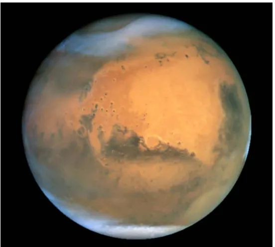
and rift valleys, such as Valles Marineris, shows geological activity that may have persisted until very recently. Its red color comes from rust in its iron-rich soil (Figure 1.2). Mars has two tiny natural satellites (Deimos and Phobos) thought to be captured asteroids.

(19)

[image:19.612.109.540.71.311.2]

Figure 1.1. Planets and dwarf planets of the Solar System. Sizes are to scale, but relative distances from the Sun are not [Source: NASA; http://sse.jpl.nasa.gov/planets/index.cfm].

Mars remains a high-priority target for exobiological investigations. The reason for this is the possibility that Mars and Earth experienced similar climatic conditions early in their history and that because life started on Earth, it might also have started on Mars. Then as the planets evolved, life flourished on Earth but became extinct on Mars [Haberle 1998].

Today Mars is a dry desert world, despite some signs that water may have once flowed freely across its surface. Where did the water go? Unlike Venus, Mars with a weak gravity allows an extended corona of hot light species and the escape of its lighter constituents, in its exosphere.

The Martian exosphere plays, therefore, a crucial role in the global escape of the

Martian atmosphere, and thus to the history of water on Mars [Chassefière and Leblanc 2004; Leblanc et al. 2006]. However, even today the information about the hot species that form the Martian corona of is very limited because of the lack of observational data, the only in situ measurements coming from the Viking 1 & 2 mission descents of 1976. Since then, a number of theoretical quantitative works have been reported in an attempt to describe its extended hot atomic corona. In the last 30 years, a great improvement in

(20)

the computational simulations has been made and the models tend to be more complex and accurate.

This work presents the first self-consistent 3D description of the Mars thermosphere and exosphere and studies its variation through seasons and solar activity. The evolution of the upper atmosphere (i.e. upper thermosphere and exosphere) is also investigated and

[image:20.612.187.463.297.545.2]

allows an estimate of the global loss of water over Martian history. Much of the work in this thesis appears in two papers already accepted for publication in a special issue of the refereed planetary journal Icarus [Valeille et al. 2009a, 2009b] and in two papers that have been submitted for publication in the Journal for Geophysical Research [Valeille et al. 2009c, 2009d].

Figure 1.2. View of Mars from Hubble Space Telescope on June 26, 2001. The colors have been carefully balanced to give a realistic view of Mars' hues as they might appear through a telescope [Source: NASA Image PIA03154; Image Credit: NASA and The Hubble Heritage Team (STScI/AURA); Acknowledgment: J. Bell (Cornell U.)].

(21)

I.1. Past studies

Originally the hot Martian corona was modeled using Venus as an analogy, and those simulations were extended to Mars [Nagy et al. 1981; Nagy and Cravens 1988; Nagy et

al. 1990; Hodges 2000]. The pioneering work on the hot corona and their role in the solar wind interaction with Mars [Nagy et al. 1988; Nagy and Cravens, 1988; Ip 1990; Nagy et al. 1990; Lammer and Bauer 1991; Hodges 1994; Fox and Hac 1997; Kim et al. 1998], considered the exobase as a theoretical level delimitating the collision-dominated thermosphere from the collisionless exosphere in order to take into account the change in collision regime in the flow. Calculations were conducted separately for each region in 1D spherical symmetry. The hot species energy distribution, computed by a two-stream transport model [Nagy and Banks 1970] in the thermosphere, was applied as a boundary condition at the exobase to calculate the oxygen density profile in the exosphere based on the Liouville equation [Chamberlain 1963].

The main limitation of these models is that they assume a strict separation between collision and collisionless domains, disregarding the collision transitional domain (between the collision-dominated thermosphere and the collisionless exosphere), where the momentum exchange within the flow is still important but the collision frequency is not high enough to maintain equilibrium. Moreover the escape fluxes generated do not include the exospheric production of hot species and their collisions with the thermospheric and exospheric background species, which account for a non-negligible part of the total escape rate [Hodges 2000; Valeille et al. 2009a].

A self-consistent description of the Martian upper atmosphere requires construction of a global physical model that accounts for kinetic processes of both the collisional

upper thermosphere and collisionless exosphere, but also in the collision transitional domain. Among the most recent proposed approaches, Hodges [2000] considered a thick atmospheric region where hot species are produced and collide with the background species before reaching the collisionless exospheric region beyond.

Taking into account the change in the collision regime in the flow, a number of theoretical quantitative works have been reported over the past ten years in an attempt to describe the extended hot atomic corona in 1D spherical symmetry [Lammer et al. 2000; Nagy et al. 2001; Krestyanikova and Shematovitch 2005; Cipriani et al. 2007]. However,

(22)

those studies are most often specific to the subsolar point, cannot account for the important diurnal variations, and therefore are inherently constrained to a local description of the altitude profile.

Keeping these considerations in mind, a few studies extended their 1D spherically symmetric thermosphere inputs to higher dimensions by simple extrapolation.

Distributions varying as a cosine function of Solar Zenith Angle (SZA) were first assumed to extend the inputs to 2D axisymmetry with respect to the Mars-Sun axis [Kim et al. 2001]. The inclusion of planetary rotation or diurnal tides added some 3D influences to the results [Hodges 2000; Chaufray et al. 2007]. However, while the improvements in the exosphere models were considerable, the spatial and temporal distribution of the results still presented the same limitations that were inherent in the 1D thermosphere inputs (taken from independent, and therefore non-consistent, studies), upon which they were based [Hanson et al. 1977; Nier and Mc Elroy 1977; Zhang et al. 1990; Fox 1993a; Kim et al. 1998; Krasnopolsky 2002].

It has been extensively demonstrated [e.g. Bell et al. 2007; Bougher et al. 2000, 2006, 2008, 2009a] that the thermosphere exhibits diurnal patterns (such as dynamical effects and abrupt changes in the ionosphere structure), as well as local variations (temperature and wind distributions, planet rotation, polar warming, hemispheric asymmetries) that cannot be treated by simple extrapolation of a 1D thermosphere.

Processes that shape the exosphere and the Martian hot corona originate deep in the thermosphere/ionosphere and interact with it. Therefore, independently of the complexity of the exosphere model used for calculations, the limitations are inherent to the thermosphere/ionospheric inputs employed. It is therefore highly desirable to employ a global kinetic model that includes a self-consistent description of both regions to provide a rigorous description of the exosphere, the hot corona, and the atmospheric loss.

(23)

I.2. Present study

In an effort to address this need, the initial studies couple self-consistently a 2D axisymmetric exosphere description with 3D thermosphere/ionosphere inputs by using a

combination of the Direct Simulation Monte Carlo (DSMC) kinetic model and the Mars Thermosphere General Circulation Model (MTGCM) both for modern [Valeille et al. 2009a] and ancient [Valeille et al. 2009b] Mars conditions. Without any further approximations, the MTGCM provides all the parameters needed to evaluate the state of the background thermosphere and ionosphere and the production of hot oxygen atoms at any point around the planet. Exospheric results are presented as a function of SZA.

A full 3D DSMC, which includes the coronal particles and describes the heating of the thermosphere, was thought to be computationally too expensive in the past [Leblanc and Johnson 2001]. After design of a 3D unstructured mesh and improvement of our DSMC model, a complete 3D description of both the thermosphere/ionosphere and exosphere can be accomplished within a reasonable computational timeframe. The results are presented and discussed in this study.

In addition to allowing a better understanding of the Martian neutral hot corona, a 3D study of the exosphere provides more insightful inputs for ionospheric studies, such as the local exobase and ion peak height determination, local ion production, atom-to-molecule ratio variations at the exobase, and information on the nightside where few measurements exist. All these exosphere parameters are critical for current 3D plasma models, as mentioned in various studies [Brecht 1997a, 1997b; Acuña et al. 1998; Leblanc and Johnson 2001, 2002; Ma et al. 2002, 2004; Modolo et al. 2005; Fang et al. 2008] that would in turn give more detailed results on ion loss, atmospheric sputtering,

and interaction with the solar wind in general. Also certain features, such as magnetic crustal fields, which influence ion loss [e.g. Fang et al. 2009], are localized and therefore can only be modeled in 3D.

The study of Valeille et al. [2009a] couples for the first time 3D thermospheric/ionospheric inputs [e.g. Bougher et al. 2006, 2008, 2009a] with a 2D exospheric description. It suggests, in particular, that varying Equatorial longitude and polar latitude cuts, i.e. calculations from 0° to 180° SZA along the Equator or through the Poles, present the greatest contrasts of thermospheric/ionospheric features and are

(24)

essentially the two extreme spatial dimensions of the Martian upper atmosphere environment (i.e. thermosphere/ionosphere and exosphere).

The same study quantifies not only the influence of the solar cycle, but also of seasons on the thermosphere/ionosphere and exosphere by characterizing the two extreme cases of net solar forcing for modern conditions, i.e. at the orbital position of Aphelion

for solar Low (or sometimes called minimum) activity (AL) and at the orbital position of Perihelion for solar High (or sometimes called maximum) activity (PH). Conclusions show that seasonal variations are comparable with the influence of solar activity, and that they both need to be addressed for a better understanding of the Martian upper atmosphere and its interactions with its surrounding environment.

The same approach is used to study the evolution of the thermosphere/ionosphere and exosphere over Martian history in the study of Valeille et al. [2009b]. The inclusion of dynamics shows that it plays a very important role in the heating/cooling mechanisms of the ancient thermosphere and that past 1D models, which inherently neglect dynamics [Zhang et al. 1993b; Lammer et al. 2003], may have overestimated the exospheric temperatures and therefore the structure of the upper atmosphere in general. The study of Valeille et al. [2009b] further concludes that variations due to ancient solar conditions and modern solar activity are comparable and therefore that studies of the ancient atmosphere should take into account solar low and high conditions to bracket the limiting cases (or consider a solar cycle average in the past), as suggested in the recent study of Chassefière et al. [2007].

The work of Valeille et al. [2009c] couples a 3D thermosphere/ionosphere model with a 3D exosphere code and studies spatial variations with altitude and with angular position on the planet (diurnal and local features) in the upper atmosphere. The simulation is run at fixed orbital position of equinox for solar low conditions (EL case), to allow comparison with the only in situ measurements available today from the Viking 1 and 2 mission descents [e.g. Hanson et al., 1977; Nier and Mc Elroy 1977]. It concludes that the thermospheric/ionospheric parameters exhibit local asymmetries that affect the entire structure of the upper atmosphere.

A complete description by a steady-state simulation requires two types of parameters to be investigated: spatial and temporal. So, while the study of Valeille et al. [2009c]

(25)

describes the spatial distribution of the upper atmosphere in the fixed EL case, the study of Valeille et al. [2009d] focuses on the variation of the thermosphere/ionosphere and exosphere parameters over all the principal timescales. Temporal perturbations can be distinguished by their characteristic time: short-scale (~1 hr), long-scale (~1-10 yr) and evolutionary-scale (~1 Gyr). A recent paper [Kaneda et al. 2007, 2009] indicates a

possible mechanism that can cause a short-term (about 2000-seconds period) enhancement of the hot oxygen escape rate in response to a sudden increase in the solar wind dynamic pressure.

I.3. Thesis outline

In this thesis, I am presenting the work on the Martian thermosphere/ionosphere and exosphere regions conducted during the last three years at the Atmospheric, Oceanic and Space Science department of the University of Michigan.

The purpose of this first introductory chapter is to present the current status of the scientific research on the subject and its motivations.

General analytical solutions of the description of an exosphere are first given by assuming a collisionless exosphere and particle motion in a gravitational field (Chapter II). Different velocity distributions (including thermal and suprathermal, isotropic and Maxwellian distributions) are considered at a critical level where the particles are injected. This constitutes a general mathematical approach and can be applied to any planet. These theoretical problems are also simulated in the code and provide an excellent

benchmark for validation of our code. They also provide a firm physical context for understanding some of the detailed features in the realistic but necessarily complicated model results.

Both thermospheric/ionospheric and exospheric models constituting our global approach, as well as how they are coupled, are then presented along with the main assumptions in the chemical and physical processes of the Martian upper atmosphere [Valeille et al. 2009a, 2009b, 2009c, 2009d] (Chapter III). Our global approach will then

(26)

9

be explained, and preliminary results on the hot oxygen production in the upper thermosphere will be discussed.

Calculations for fixed orbital position of equinox and for solar low conditions (EL case) are presented and discussed (Chapter IV). These specific conditions (corresponding to Viking measurements) have been systematically used in the past by modelers and

serve as an example to illustrate the general structure and attributes of a 3D exosphere produced by a self-consistent 3D thermosphere/ionosphere model [Valeille et al. 2009a, 2009c]. Comparisons with other relevant studies of the last ten years are also presented.

Modern long-term periodic variations (timescales of about 1-10 yr) are first investigated (Chapter V). Along with the expected variability of the hot oxygen corona with solar cycle, this study is the first to show that differences in the results in general, and in the escape fluxes specifically, are important between the different orbital positions considered: equinox, perihelion and aphelion. These season driven variations are of the same order as solar cycle driven variations [Valeille et al. 2009a, 2009d].

The loss of water from Mars can be evaluated by studying the evolution of the escape rate of atomic oxygen over time (Chapter VI). Throughout Martian history, the evolution of solar radiation has led to significant variations in the macroscopic parameters of the thermosphere/ionosphere, which in turn governs the hot species population of the exosphere and especially the atmospheric loss rates [Valeille et al. 2009b, 2009d].

Secondary processes of creation of hot atomic oxygen (O), as well as the population and escape of other neutral exospheric hot species, such as hydrogen (H) and carbon (C), are investigated in a preliminary way. Future work is also discussed (Chapter VII).

(27)

10

Chapter II

Ballistic motion of a particle in a gravitational field in spherical

coordinates

In this chapter, a general analytical solution of the description of an exosphere is given by considering the motion of a single particle in the gravitational field of a spherical body in a collisionless domain. This mathematical approach can be applied for any body and for any particle independently of its energy (thermal or non-thermal).

The case of Mars will be used for numerical applications and illustration purpose in the remainder of this chapter. These assumptions are reasonable in the particular example of Mars as long as the domain of study is situated within a lower boundary, above which the particles flow can be characterized as collisionless, and an upper boundary, above which the gravitational field of other celestial bodies has to be taken into account and where the two-body approximation is no longer valid.

This theoretical exercise provides a solid benchmark for the most important processes of the exospheric code, which will be presented in detail in the next chapter and used all along this study in order to obtain a better understanding of the Martian upper atmosphere.

II.1. Equation of motion

In spherical coordinates (C, er, eΘ, eΦ), with the center C of the planet taken as origin,

the position, r, of a particle is written,

(28)

11 Its velocity, v, is then, by differentiation,

𝑣 =𝑑𝑟 _𝑑𝑡 = 𝑟 𝑒 _𝑟 + 𝑟Θ 𝑒 _Θ + 𝑟sin Θ Φ 𝑒 _Φ (2.2)

Its acceleration, a, is therefore,

𝑎 =𝑑

2_𝑟

𝑑𝑡2 =

𝑟 − 𝑟Θ 2 _{− 𝑟sin}2_{Θ Φ}2_𝑒 𝑟 2𝑟 Θ + 𝑟Θ + 𝑟sin Θ cos Θ Φ 2_𝑒

Θ 2 𝑟 sin ΘΦ + 2𝑟 cos Θ Θ Φ + 𝑟sin ΘΦ 𝑒 _Φ

(2.3)

Furthermore, the derivative of the angular momentum, L, is,

𝑑𝐿 _𝑑𝑡 =𝑑𝑟 _𝑑𝑡 × 𝑚𝑣 + 𝑟 × 𝑚𝑑𝑣 _𝑑𝑡 = 0 + 𝑟 × 𝑚𝑎 (2.4) where m is the mass of the particle.

The gravity g of the planet, which is assumed to be the only force that acts on the particle, is radial. Newton’s law then gives,

𝑚𝑎 = 𝑚𝑔 𝑟 = −𝑚_𝑟𝜇₂𝑒 _𝑟 (2.5) where μ = GM, is the standard gravitational parameter, with G, gravitational constant (~ 6.67 x 10-11 m3 kg-1 s-2) and M, mass of the planet (for Mars, it would be M ~ 6.42 x 1023 kg and then μ ~ 4.28 x 1013 m3 s-2).

It follows that the angular momentum L is conserved,

𝑑𝐿 _𝑑𝑡 = −𝑚𝜇_𝑟 𝑒 _𝑟 ∧ 𝑒 _𝑟 = 0 (2.6) leading to,

𝐿 𝑟 = 𝑟 × 𝑚𝑣 = 0 −𝑚𝑟𝑣Φ 𝑟

𝑚𝑟𝑣_Θ 𝑟 = 𝐿 𝑟 0 = 𝑟 0× 𝑚𝑣 0 =

0 −𝑚𝑟₀𝑣_Φ₀ 𝑟 ₀

𝑚𝑟₀𝑣_Θ₀ 𝑟 0

(2.7)

where v and v0 are the particle velocity at the current and initial position r and r0,

respectively. The position r0, where the particle is initially injected with the velocity v0, is

situated at a critical level r0, above which it is assumed that there are no collisions, no source and no sink of particles.

With these relations of conservation, and defining the perpendicular speed as, 𝑣_⊥2 = 𝑣_Θ2+ 𝑣_Φ2 (2.8) Equation (2.3) can be rewritten with expressions (2.7) and (2.8),

𝑚𝑎 = 𝑚 𝑟 −𝑟0

2_𝑣 ⊥02

(29)

12 And Newton’s law (2.5) becomes,

𝑟 =𝑟0

2_𝑣 ⊥02 𝑟3 −

𝜇

𝑟2 (2.10)

II.2. Escaping and non-escaping particles

The particles can be divided in two exclusive groups: the escaping and non-escaping particles. The escaping particles are the ones with sufficient initial speed v0 to "break free" from the gravitational field without any additional impulse (i.e. so that gravity will never manage to pull it back). This definition results in a condition on v0 expressed via the equation of conservation of energy E(r), obtained by integrating Newton’s law (2.5) over the infinitesimal element dr from r0 to ∞,

𝐸 𝑟₀ =1₂𝑚𝑣₀2− 𝑚_𝑟𝜇

02 = 𝐸 ∞ = 1

2𝑚𝑣∞2 ≥ 0 (2.11)

The minimum initial speed v0 that satisfies this inequality is obtained for v∞ = 0 and is equal to and defines the escape speed vesc,

𝑣𝑒𝑠𝑐 𝑟 = 2𝜇 𝑟 (2.12)

the speed where the kinetic energy of an object is equal to the magnitude of its gravitational potential energy. Escape speed is independent of the mass of the particle. It depends only on the mass M of the planet and the distance where it is calculated. For illustration purpose, escape speeds for each planet of the solar system are presented in Table 2.1. Calculations are made either at the surface of the planet (for terrestrial inner planets) or at the altitude corresponding to a local pressure of 1 atm (for gas giant outer planets).

(30)

13

It is important to note that the general frame (C, ex, ey, ez) of this study is fixed by

pointing towards arbitrary fixed stars and that steady-state is assumed. Therefore, initial conditions can be different for a particle defined in the frame associated with the planet. In this particular case, planetary rotation has to be taken into account, and the escape speed relative to the surface of a rotating body depends on direction, in which the escaping body travels. The surface speed decreases with the cosine of the geographic latitude, and this is the reason why space launch facilities are often located as close to the Equator as feasible (e.g. the American Cape Canaveral in Florida and the European Guiana Space Centre, only 5° from the Equator in French Guiana).

For simplicity sake, the frame of study adopted in this chapter is the general frame as defined above. Most of past works on Mars exosphere are either one- or two-dimensional and therefore can inherently account for neither planetary rotation nor winds. These parameters play however an important role on determining the initial speed v0 of a particle and therefore affect its entire motion. Their effects will be treated in the following chapters.

II.3. Maximum altitude reached by non-escaping particles

While escaping particles have sufficient initial speed to escape the gravitational field of the planet, other particles (with v0 < vesc) are trapped in the gravitational field and will come back eventually to their initial altitude r0.

Conservation of energy (2.11) can also be obtained after multiplying both sides of Equation (2.10) by r and integrating between time t, where the particle is at r and t0 where it was at r0,

𝑟

2

2 − 𝑟 02

2 = − 𝑟02𝑣_⊥02

2 1 𝑟2−

1

𝑟₀2 + 𝜇 1 𝑟−

1

𝑟0 (2.13)

Using the expression of vesc from Equation (2.11), and defining the angle θ0 on [0, π/2] of the vector v0 with respect to the local vertical (i.e. radial direction) er,

𝑟 2 = 𝑣₀2cos2𝜃₀− 𝑣₀2sin2𝜃₀ 𝑟0

2

𝑟2− 1 + 𝑣𝑒𝑠𝑐2 𝑟0 𝑟0

(31)

14

The domain of definition D of this equation is D = [r0, ∞[ for escaping particles, but is D = [r0, rmax] and finite for non-escaping particles.

rmax is the maximum distance from the center of the planet they reach before they fall back down ballistically towards the critical level r0. It corresponds to r0 in Equation (2.13), and by writing a = r0/r on ]0, 1], is the solution of the quadratic equation,

sin2𝜃₀𝑎2− 𝑋₀𝑎 + 𝑋₀− 1 = 0 (2.15) where X0 = (vesc(r0)/ v0)2 is the escape parameter, square of the ratio of the escape speed over the particle speed at the critical level r0. It is strictly positive (X0 ]0, ∞[) and allows to make the distinction between non-escaping particles (X0 > 1), and escaping particles (X0 ≤ 1). It equals 1 at the local escape speed (i.e. v0 = vesc(r0)) and commonly used with the most probable speed (i.e. v0 = vth(r0)) to quantify, for instance, Jeans escape. The trivial case (v0 = 0) will be put aside in the remaining of this chapter (for the sake of X0 definition).

For θ0 ≠ 0 and v0 ≠ 0, the roots a- and a+ of Equation (2.15) are,

𝑎_±=

𝑋0± 𝑋02−4 sin2𝜃0 𝑋0−1

2 sin2_𝜃

0 (2.16)

For non-escaping particles, only one root is acceptable within the domain of definition of a. By multiplying numerator and denominator by denominator conjugate expression, rmax can be written,

𝑟_𝑚𝑎𝑥 𝑟₀, 𝑣 ₀ =

𝑋0+ 𝑋02−4 sin2𝜃0 𝑋0−1

2 𝑋0−1 𝑟0 (2.17)

(32)

15

[image:32.612.171.480.136.390.2]

represented corresponding to the respective 3D and 2D simulation domains presented in the next chapter.

Figure 2.1. Maximum altitude reached by non-escaping particles. The two black vertical lines correspond to vesc(r0) and vesc(r0)/√2.

For an initially purely perpendicular particle, two cases must be considered, If 0 ≤ 𝑣₀ ≤ 𝑣_𝑒𝑠𝑐 𝑟₀ 2,

𝑟_𝑚𝑎𝑥 𝑟₀, 𝑣 ₀ = 𝑟₀ (2.19) If 𝑣_𝑒𝑠𝑐 𝑟₀ 2≤ 𝑣₀ < 𝑣_𝑒𝑠𝑐 𝑟₀ ,

𝑟_𝑚𝑎𝑥 𝑟₀, 𝑣 ₀ =_𝑋1

0−1𝑟0 (2.20)

(33)

16

Figure 2.2. Family of elliptical satellite orbits.

II.4. Velocity profile

From Equations (2.7) and (2.14), the velocity can be written, on the same respective domain of definition D,

𝑣 𝑟 =

𝑣0 1 − 𝑟0_𝑟 sin 𝜃0 2

− 𝑋₀ 1 −𝑟0_𝑟 𝑒 _𝑟 𝑟0

𝑟 𝑣𝜃0 𝑟 0 𝑒 𝜃 𝑟0

𝑟 𝑣𝜑0 𝑟 0 𝑒 𝜑

(2.21)

The speed v can then be written,

𝑣 𝑟 = 𝑣₀2− 𝑣_𝑒𝑠𝑐2 𝑟₀ − 𝑣_𝑒𝑠𝑐2 𝑟 (2.22)

For escaping particle, the velocity becomes radial and reaches saturation,

lim𝑟→∞𝑣 𝑟 = 𝑣∞𝑒 𝑟 = 𝑣02− 𝑣𝑒𝑠𝑐2 𝑟0 𝑒 𝑟 (2.23)

corresponding to the asymptote on Figure 2.3 (black line). More precisely, with a Taylor expansion of first order on r0/r,

𝑣 𝑟 ~_𝑟→∞𝑣_∞𝑒 _𝑟 +𝑟_𝑟0𝑣 _𝑐𝑜𝑟 + 𝑂 𝑟_𝑟0

2

(2.24)

with,

𝑣 _𝑐𝑜𝑟 =1₂𝑣𝑒𝑠𝑐

2 _𝑟 0

(34)

17

Figure 2.3. Radial component of the velocity for non-escaping (a) and escaping (b) particles for various initial pitch angle θ0. The black vertical line in (b) corresponds to v∞.

[image:34.612.155.492.92.406.2]

(35)

18

II.5. Time of flight and angular displacement

II.5.1. Time of flight

With different initial speeds v0 and directions θ0, particles will spend a different time t0 (from a very wide range) in the domain of study. A particle exits the domain of study when it crosses the upper boundary, rext, or the lower boundary, r0. It is important to note that because the domain of study is finite, particles that exit the domain at the upper boundary are escaping particles and nearly-escaping particles, i.e. non-escaping particles that have a maximum altitude above the upper limit (rmax > rext). The study of the time of flight t0 allows a better understanding of the ionization and collision processes in the exosphere/upper-ionosphere. Indeed, for instance, the probability of photoionization of a particle, pPI, is proportional to the time t0 spent by the particle in the system,

𝑝_𝑃𝐼 = 1 − 𝑒−

𝑡0 𝑡𝑃𝐼_~ 𝑡0

𝑡𝑃𝐼 (2.26)

where tPI is the local photoionization time (increasing with increasing heliocentric distance), and tPI >> t0. In the same way, a probability of collision could be estimated.

For escaping and nearly-escaping particles, the time of flight in the system is given by,

𝑡₀ = 𝑡 𝑟₀, 𝑣 ₀ = _𝑣𝑑𝑟

∥ 𝑟 𝑟𝑒𝑥𝑡

𝑟0 (2.27)

For non-escaping particles, the time of flight in the system is given by, 𝑡₀ = 𝑡 𝑟₀, 𝑣 ₀ = 2 _𝑣𝑑𝑟

∥ 𝑟 𝑟𝑚𝑎𝑥

𝑟0 (2.28)

With the expression of the radial velocity (2.21), the identities (2.27) and (2.28) can be rewritten, respectively,

𝑡₀ =_𝑣1

0

𝑟𝑑𝑟

− 𝑟0sin 𝜃0 2+ 𝑋0𝑟0 𝑟+ 1−𝑋0 𝑟2 𝑟𝑒𝑥𝑡

𝑟0 (2.29)

𝑡₀ =_𝑣2

0

𝑟𝑑𝑟

− 𝑟0sin 𝜃0 2+ 𝑋0𝑟0 𝑟+ 1−𝑋0 𝑟2 𝑟𝑚𝑎𝑥

𝑟0 (2.30)

(36)

19

Figure 2.4. Time of flight in a 3-Martian-radius domain of study for particles with initial speed v0 up to 6.0 km s-1.

II.5.2. Angular displacement and deviation

II.5.2.1. Angular displacement

Similarly, with different initial speeds v0 and directions θ0, particles undergo different angular displacements β0 in their motion in the domain of study. β0 is the angle between the position where the particle is injected initially and the final position where the particle exits the system. This is particularly important to understand (in a 2D axisymmetric simulation for instance) the apparent paradox of a nightside population in a problem where particles are created on the dayside of the planet only.

For escaping and nearly-escaping particles, the angular displacement in the system is given by,

𝛽0 = 𝛽 𝑟0, 𝑣 0 = 𝑣⊥0 𝑟_𝑟02 𝑟0𝑑𝑡 𝑟𝑒𝑥𝑡

𝑟0 (2.31)

For non-escaping particles, the angular displacement in the system is given by,

𝛽0 = 𝛽 𝑟0, 𝑣 0 = 2 𝑣⊥0 𝑟_𝑟02 𝑟0𝑑𝑡 𝑟𝑚𝑎𝑥

𝑟0 (2.32)

With the expression of the radial velocity (2.21), the identities (2.27) and (2.28) can be rewritten, respectively,

𝛽₀ = 𝑟₀sin 𝜃₀ 𝑑𝑟

𝑟 − 𝑟0sin 𝜃0 2+ 𝑋0𝑟0 𝑟+ 1−𝑋0 𝑟2 𝑟𝑒𝑥𝑡

𝑟0 (2.33)

𝛽0 = 2 𝑟0sin 𝜃0 _{𝑟 − 𝑟0}_{sin 𝜃0} 2_{+ 𝑋0𝑟0 𝑟+ 1−𝑋0 𝑟}𝑑𝑟 2 𝑟𝑚𝑎𝑥

(37)

20

Figure 2.5a shows the angular displacement β0 for particles with different initial speeds v0 and directions θ0 (in solid lines) for a 3-Martian-radius domain.

II.5.2.2. Angular deviation

The angle of deviation Δβ is defined in this study as the differential effect of an additional perpendicular push, vadd, added to the initial velocity, v0, of a particle, i.e., ∆𝛽 = 𝛽₁− 𝛽₀ = 𝛽 𝑟₀, 𝑣 ₀+ 𝑣 _𝑎𝑑𝑑 − 𝛽 𝑟₀, 𝑣 ₀ (2.35)

This constitutes the theoretical explanation of the effect of thermospheric winds and/or planetary rotation on the exospheric distribution of a celestial body.

Figure 2.5a shows (in dashed lines) the angular displacement β1 due to an additional perpendicular push of vadd = vPR = 240 m s-1 added to the initial velocity, v0, of a particle in a 3-Martian-radius domain. This corresponds to the Equatorial rotation speed at the Martian surface. Horizontal thermospheric wind speeds would be about twice faster (vadd = vTW ~ 500 m s-1). Because the two effects are in opposite directions (on Mars, planetary rotation is directed towards east, whereas thermospheric winds are towards west), their cumulative effect is somewhat similar to the planetary rotation alone (vadd = vTW - vPR ~ vPR). The angular deviation Δβ due to the planetary rotation is presented in Figure 2.5b.

(38)

21

II.6. Density profile

II.6.1. General case

According to Liouville’s theorem, one can write,

𝑓 𝑟 , 𝑣 = 𝑓 𝑟 ₀, 𝑣 ₀ (2.36) where f is the velocity distribution function in spherical coordinates. This asserts that the phase-space distribution function is constant along the trajectories of the system - that is that the density of system points in the vicinity of a given system point travelling through phase-space is constant with time.

For simplicity sake, a uniform distribution of injected particles all around the planet relative to the initial position r0 in the spatial frame (r, Θ, Φ) is used here. By symmetry

of the problem, all expressions in the remainder of this chapter are then functions of the scalar distance, r, rather than the vector position, r.

The conservation of energy (2.13) and angular momentum (2.7) relations give the relationships between v, v0, θ and θ0,

𝑣

2_{− 𝑣}

𝑒𝑠𝑐2 𝑟 = 𝑣02− 𝑣𝑒𝑠𝑐2 𝑟0

𝑟𝑣 sin 𝜃 = 𝑟₀𝑣₀sin 𝜃₀ (2.37)

Decoupling this 𝑣, 𝜃 ; 𝑣₀, 𝜃₀ system leads to the following relations,

𝑣 𝑟 = 𝑣₀2 _{− 𝑣}

𝑒𝑠𝑐2 𝑟0 − 𝑣𝑒𝑠𝑐2 𝑟

sin 𝜃 = 𝑣0

𝑣₀2_{− 𝑣}

𝑒𝑠𝑐2 𝑟0 −𝑣𝑒𝑠𝑐2 𝑟 𝑟0

𝑟 sin 𝜃0

(2.38)

The density n(r) at the position, r, can then be written,

𝑛 𝑟 = 𝜀 ₀∞ ₀2𝜋 ₀𝜋 2𝑓 𝑟, 𝑣 𝛿3𝑣

= 𝜀 ₀∞ ₀2𝜋 ₀𝜋 2𝑓 𝑟, 𝑣 𝑣2sin 𝜃 𝑑𝑣𝑑𝜃𝑑𝜑 (2.39) The factor ε equals 1 when the density, n(r), refers to escaping particles, whereas it equals 2 for non-escaping particles. Indeed, escaping particles are only moving in the upward direction away from the planet (θ < π/2), whereas (for an infinitesimal volume in the domain of definition) half of the non-escaping are moving away from the planet (θ < π/2) and the other half towards the planet (θ > π/2).

(39)

22

isotropic (half the population moving upward, half the population moving downward), whereas above it, all the population is moving upward.

Rewriting relation (2.34) exclusively in term of the initial conditions leads to,

𝑛 𝑟 = 𝜀 _𝑣 𝑓 𝑟₀, 𝑣 ₀ |𝐽_{𝑣 𝑣}₀ | 𝑣2sin 𝜃 𝑑𝑣₀𝑑𝜃₀𝑑𝜑₀

0𝜖𝐷𝑒𝑓𝐽 (2.40)

where |𝐽_{𝑣 𝑣 0} | is the determinant of the Jacobian matrix from the current frame R to the initial frame R0. 𝐷𝑒𝑓𝐽 is the domain of definition of 𝐽𝑣 𝑣 0 . For a non-escaping particle, it

includes the condition that at any altitude level, the particle must have an upward velocity of zero (corresponding to rmax) or greater (below rmax). It is also important to note that v does not depend on θ0.

𝐽_{𝑣 𝑣 0} = _𝜕𝑣𝜕𝑣

0× 𝜕𝜃 𝜕𝜃0 =

𝑟0𝑣02cos 𝜃0

𝑟𝑣2_{cos 𝜃} (2.41)

With Equation (2.36), part of the expression in the integral in (2.35) can be developed to,

𝑣2sin 𝜃 𝐽_{𝑣 𝑣 0} =𝑟0𝑣0

2_{cos 𝜃} 0

𝑟 tan 𝜃

=𝑟0𝑣0

2_{cos 𝜃0}

𝑟

𝑟0𝑣0sin 𝜃0 𝑟2_𝑣2_{− 𝑟}

0𝑣0sin 𝜃0 2

=𝑟0

2

𝑟2

𝑣02cos 𝜃0sin 𝜃0

1− 𝑟0_𝑟 sin 𝜃0 2

−𝑣𝑒𝑠𝑐2 𝑟0 𝑣02 1−

𝑟0 𝑟

(2.42)

And, using the above definition of the escape parameter, X0, the expression of the density (2.35) can be simplified to,

𝑛 𝑟 = 𝜀𝑟0

2

𝑟2

𝑓 𝑟0,𝑣 0 𝑣02cos 𝜃0sin 𝜃0

1− 𝑟0_𝑟 sin 𝜃0 2

−𝑋0 1−𝑟0_𝑟

𝑑𝑣₀𝑑𝜃₀𝑑𝜑₀

𝑣 0𝜖𝐷𝑒𝑓𝐽 (2.43)

Given Equation (2.38), the density, n(r), at a location, r, can be calculated if the velocity distribution function, f(r0, v0), is known. Analytic expressions for n(r) are obtained

assuming various distributions at the critical level r0.

II.6.2. Constant initial velocity v0

If all particles are injected with the same upward velocity v0 = v0’ (θ < π/2), the

velocity distribution function is, at r0,

𝑓 𝑟₀, 𝑣 ₀ 𝑣₀2sin 𝜃₀ =𝑛 𝑟0

2 𝛿(𝑣0− 𝑣0 ′_)𝛿(𝜃

(40)

23

The factor ½ comes again from the above assumption that below the level r0, half of the particles move upward (and then are actually injected in the domain of study) and half of them move downward. This assumption is made for the sake of the continuity in the densities of returning particles. δ is the Dirac delta function, defined as,

𝛿 𝑥 = ∞ 𝑓𝑜𝑟 𝑥 = 0_{0 𝑓𝑜𝑟 𝑥 ≠ 0} (2.45)

and which is also constrained to satisfy the identity,

_−∞+∞𝛿(𝑥)𝑑𝑥 = 1 (2.46) Expressions (2.35) and (2.36) lead then to,

𝑛 𝑟 = 𝜀𝑛 𝑟₀ 𝑟0

2

𝑟2

cos 𝜃0𝛿(𝑣0−𝑣0′)𝛿(𝜃0−𝜃0′)𝛿(𝜑0−𝜑0′)

1− 𝑟0_𝑟 sin 𝜃0 2

−𝑋0 1−𝑟0_𝑟

𝑑𝑣0𝑑𝜃0𝑑𝜑0 𝑣 0𝜖𝐷𝑒𝑓𝐽

=₂𝜀𝑛 𝑟0 𝑟0 2

𝑟2

cos 𝜃0

1− 𝑟0_𝑟 sin 𝜃0 2−𝑋0 1−𝑟0_𝑟

(2.47)

This expression could also have been obtained by using the conservation of the upward flux between r0 and r, in the limit of the domain of definition,

4𝜋𝑟2𝑣∥ 𝑟 𝑛 𝑟 = 2𝜀𝜋𝑟02𝑣∥ 𝑟0 𝑛 𝑟0 (2.48)

For the particular case of radial injection (θ0’ = 0) of non-escaping particles (ε = 2), the expression (2.38) becomes,

𝑛 𝑟 = 𝑛 𝑟₀ 𝑟0

2

𝑟2 1

1−𝑋0 1−𝑟0_𝑟

(2.49)

(41)

[image:41.612.198.454.74.328.2]

24

Figure 2.6. Density profile for radial non-escaping particles computed by 1D (a) and 2D (b) spherical simulations. Results from the simulation (a, red dashed line) can be compared with the theory (a, blue solid line).

II.6.3. Isotropic distribution (constant initial speed v0)

If all particles are injected isotropically into the upward 2π steradian with the same upward speed v0 = v0’, the velocity distribution function is, at r0,

𝑓 𝑟0, 𝑣 0 =𝛿(𝑣0−𝑣0 ′₎

4𝜋𝑣02 𝑛 𝑟0 (2.50)

Expressions (2.35) and (2.36) lead then to,

𝑛 𝑟 =𝜀𝑛 𝑟_4𝜋0 𝑟0

2

𝑟2

𝛿(𝑣0−𝑣0′) cos 𝜃0sin 𝜃0

1− 𝑟0_𝑟 sin 𝜃0 2−𝑋0 1−𝑟0_𝑟

𝑑𝑣0𝑑𝜃0𝑑𝜑0 𝑣 0𝜖𝐷𝑒𝑓𝐽

=𝜀₂𝑟0

2

𝑟2𝑛 𝑟0

sin 𝜃0cos 𝜃0

1− 𝑟0_𝑟 sin 𝜃0 2−𝑋0 1−𝑟0_𝑟 𝑑𝜃0 𝜃𝑙𝑖𝑚(𝑟)

0 (2.51)

where θlim, function of r and the initial state (r0, v0), is the initial angle of a particle that

reaches its maximum altitude at r (i.e. for which r = rmax(r0, v0)). It is defined, for

(42)

25 𝜃_𝑙𝑖𝑚(𝑟) = arcsin _𝑟𝑟

0 1 − 𝑋0 1 − 𝑟0

𝑟

= arcsin _𝑟𝑟

0 𝑟𝑙𝑖𝑚−𝑟

𝑟𝑙𝑖𝑚−𝑟0 (2.52)

For escaping particle, θlim is constant and equals π/2.

With the change of variable 𝑠 = sin 𝜃0 monotonic from 0, 𝜃𝑙𝑖𝑚 𝑟 ∁ 0, 𝜋 2 to 0, sin 𝜃𝑙𝑖𝑚 𝑟 ∁ 0,1 , (2.28) becomes,

𝑛 𝑟 =𝜀

2 𝑟02

𝑟2𝑛 𝑟0

𝑠

1− 𝑟0_𝑟𝑠 2−𝑋0 1−𝑟0_𝑟 𝑑𝑠 sin 𝜃𝑙𝑖𝑚 𝑟

0 (2.53)

II.6.3.1. For non-escaping particles

With 𝐴_𝑟2 = 1 − 𝑋₀ 1 −𝑟_𝑟0 = 𝑟_𝑟0sin 𝜃_𝑙𝑖𝑚 𝑟

2

and the change of variable 𝑦 =

𝑟0 𝑟

𝑠 𝐴𝑟 =

𝑠

sin 𝜃𝑙𝑖𝑚 𝑟 monotonic from 0, sin 𝜃𝑙𝑖𝑚 𝑟 ∁ 0,1 to 0,1 ,

𝑛 𝑟 = 𝑛 𝑟₀ 𝐴_𝑟 𝑦

1−𝑦2𝑑𝑦 1

0 (2.54)

With the change of variable 𝑧 = arcsin y monotonic from 0,1 to 0, 𝜋 2 when

𝑟0

𝑟 ≤ 𝐴𝑟, i.e. when 𝑟 ≥ 𝑟𝑙𝑖𝑚 − 𝑟0,

𝑛 𝑟 = 𝐴_𝑟𝑛 𝑟₀ ₀𝜋 2sin 𝑧 𝑑𝑧 = 𝐴_𝑟𝑛 𝑟₀ (2.55) When 𝑟 = 𝑟₀, 𝐴_𝑟 = 1, and 𝑛 𝑟 = 𝑛 𝑟₀ .

And, as lim_{𝑟→𝑟𝑙𝑖𝑚} 𝐴_𝑟 = 0, we found lim_{𝑟→𝑟𝑙𝑖𝑚} 𝑛 𝑟 = 0,

𝑛 𝑟 = 1 − 𝑋₀ 1 −𝑟_𝑟0 𝑛 𝑟₀ (2.56)

(43)

26

Figure 2.7. Density profile of an isotropic injection of non-escaping particles at the critical level r0.

II.6.3.2. For escaping particles

With 𝐴_𝑟2 = 1 − 𝑋₀ 1 −𝑟0

𝑟 and the change of variable 𝑌 = 𝑟0

𝑟 𝑠

𝐴𝑟monotonic from 0,1

to 0,𝑟0

𝑟 1 𝐴𝑟 ∁ 0,

1

𝐴_𝑟0 = 0,1 ,

𝑛 𝑟 =1₂𝑛 𝑟₀ 𝐴_𝑟 𝑦

1−𝑦2𝑑𝑦 𝑟0

𝑟 1 𝐴𝑟

0 (2.57)

With the change of variable 𝑧 = arcsin y monotonic from 0,𝑟_𝑟0_𝐴1

𝑟 ∁ 0,1 to 0, arcsin 𝑟0_𝑟 _𝐴1

𝑟 ∁ 0, 𝜋 2 ,

𝑛 𝑟 =1

2𝑛 𝑟0 𝐴𝑟 sin 𝑧 𝑑𝑧

arcsin 𝑟_𝑟0_𝐴1 𝑟

0

𝑛 𝑟 =1₂𝐴_𝑟 1 − 1 − 𝑟_𝑟0_𝐴1

𝑟 2

𝑛 𝑟₀ (2.58)

When 𝑟 = 𝑟₀, 𝐴_𝑟₀ = 1, and 𝑛 𝑟 =1

(44)

27

With 𝐴_∞ = lim_𝑟→∞𝐴_𝑟 = 1 − 𝑋₀, the expression of the density n(r) can be found,

lim_𝑟→∞𝑛 𝑟 ~𝑛 𝑟0_2𝐴

∞ 𝑟0

𝑟 2

(2.59)

This result can be also found by conservation of the normal flux and the asymptotic expression of the velocity (2.23).

[image:44.612.198.447.242.444.2]

Figure 2.8 shows a hypothetical density profile of an isotropic injection (n0 = 105 cm-3) for r0 corresponding to an altitude of 200 km for non-escaping particles (v0 = 6 km s-1) at Mars. It can be compared with Figure 2.7.

Figure 2.8. Density profile of an isotropic injection of escaping particles at the critical level r0.

II.6.4. Thermal (Maxwellian) distribution

Finally, a Maxwellian velocity distribution is assumed for the base of the domain of study, which ejects particles in it. The density distribution is then calculated numerically.

𝑓 𝑟 0, 𝑣 0 = 8𝜋2𝑟02 _{2𝜋𝑘𝑇}𝑚 3 2

𝑛 𝑟0 𝑒−𝑚/2𝑘𝑇𝑣0 2

𝑣2_{sin 𝜃 𝑑𝑣}

0𝑑𝜃0𝑑𝜑0 (2.60)

The green line represented in Figure 2.9 would be the density profile for a Maxwellian distribution in a thick isothermal atmosphere. Its expression is given by the barometric formula,

(45)

28 with,

𝐸 = 𝑟0

𝐻0 (2.62)

where H0 is the scale height at r0,

𝐻₀ = 𝐻 𝑟₀ = 𝑘𝑇0

𝑚𝑔0 (2.63)

If it is assumed that there is no collision above the critical level r0, the density profile would be [see Opik and Singer 1959, 1961; Shen 1963],

𝑛_𝑇 𝑟 = 𝑛_𝑕 𝑟 − 𝑛_𝑐 𝑟 (2.64) with,

𝑛_𝑐 𝑟 = 𝑛₀ 1 − 𝑟0_𝑟

2 𝑒−

𝐸 1+𝑟0_𝑟

(2.65)

nT differs from the barometric formula (2.61) by a term nc(r). This term nC is zero when r = r0, it increases with r, and its asymptotic value is n0e-E. Note that nT gives zero density at infinity, which is different from that obtained assuming hydrostatic approximation.

Finally, if it is taken into account that the escaping particles were counted twice, the density profile is written,

𝑛_𝑎 𝑟 = 𝑛_𝑇 𝑟 − 𝑛_𝑠 𝑟 (2.66) with,

𝑛_𝑠 𝑟 = 𝑛₀

𝑟0 𝑟

2

2 𝜋𝐸

1+𝐸 𝑒−𝐸

𝐻 𝐸 −1+ 1−2₃𝐻 𝐸 𝑟0_𝑟 (2.67)

where,

𝐻 𝐸 ~

𝐸→∞1 + 2

𝐸 (2.68)

(46)

29

Figure 2.9. Density profiles of a thermal injection of particles at a critical level r0. The numerical results (red dashed line) are compared to the theory for collision and collisionless domains (blue solid line and green dashed-dotted line, respectively). Parameters are set for hydrogen in EL conditions (n0 = 3.95 x 105 cm-3, T0 = 200 K, r0 corresponding to an altitude of 200 km).

(47)

Chapter III

Model and assumptions

In this chapter, both thermospheric/ionospheric and exospheric models used together in our approach, as well as how they are coupled, are presented. The main assumptions in the chemical and physical processes of the Martian upper atmosphere [Valeille et al. 2009a, 2009b, 2009c, 2009d] are described. Our global approach is then explained and preliminary results on the hot oxygen production in the upper thermosphere are discussed.

III.1. Thermosphere/ionosphere models

III.1.1. 1D thermosphere/ionosphere models

Even today the information about Mars upper atmosphere is very limited because of the lack of observational data, the only in situ measurements coming from the Viking 1 & 2 mission descents of 1976 (Figures 3.1a and 3.1b).

Neutral mass spectrometers carried on the aeroshells of Viking 1 and Viking 2 ind