R E S E A R C H
Open Access
A new reweighted
l
minimization algorithm
for image deblurring
Tiantian Qiao
1,2*, Boying Wu
2, Weiguo Li
1and Alun Dong
1*Correspondence:
1College of Science, China
University of Petroleum, Changjiangxi Road 66, Qingdao, 266580, P.R. China
2Department of Mathematics,
Harbin Institute of Technology, West Dazhi Street 92, Haerbin, 150001, P.R. China
Abstract
In this paper, a new reweightedl1minimization algorithm for image deblurring is
proposed. The algorithm is based on a generalized inverse iteration and linearized Bregman iteration, which is used for the weightedl1minimization problem
minu∈Rn{uω:Au=f}. In the computing process, the effective using of signal information can make up the detailed features of image, which may be lost in the deblurring process. Numerical experiments confirm that the new reweighted algorithm for image restoration is effective and competitive to the recent state-of-the-art algorithms.
Keywords: reweightedl1minimization; generalized inverse; linearized Bregman
iteration; image deblurring
1 Introduction
Image deblurring is a fundamental problem in image processing, since many real-life prob-lems can be modeled as deblurring probprob-lems []. In this paper, a new reweightedl mini-mization algorithm for image deblurring is proposed. The algorithm is obtained based on a generalized inverse iteration and a linearized Bregman iteration.
Simply, we shall denote images as vectors in Rn by concatenating their columns. Let
u∈Rnbe the underlying image. Then the observed blurred imagef ∈Rnis given by
f =Au+η, (.)
whereη∈Rnis an additive noise andA∈Rm×nis a linear blurring operator. This problem is ill-posed due to the large condition number of the matrixA. Any small perturbation on the observed blurred imagef may cause the direct solutionA–f, which is very difficult to obtain from the original imageu[]. This is a widely studied subject and many correspond-ing approaches have been developed, and one of them is to minimize some cost functionals []. The simplest method is a Tikhonov regularization, which minimizes an energy con-sisting of a data fidelity term and anlnorm regularization term.Ais a convolution, which can solve the problem in the Fourier domain. In this case, the method is called a Wiener filter [], this is a linear method, and the edges of restored image are usually smeared. To overcome this, a total variation (TV)-based regularization was proposed by Rudinet al.
in [], which is known as the ROF model. Due to its virtue of preserving edges, it is widely used in image processing, such as blind deconvolution, inpainting, and superresolution; see []. However, as we know, for the TV yields staircasing [, ], these TV-based methods
do not preserve the fine structures, details, and textures. To avoid these drawbacks, non-local methods were proposed for denoising [, ], and then extended to deblurring []. Also, the Bregman iteration, introduced to image science [], was shown to improve TV-based blind deconvolution [–]. Recently, a nonlocal TV regularization was invented based on graph theory [] and applied to image deblurring []. Another approach for deblurring is the wavelet-based method,etc.[].
Normally, the original imageu∈Rnwill be found by solving the following constrained
minimization problem:
min
u∈Rn
J(u) :Au=f, (.)
whereJ(u) is a continuous convex function, and whenJ(u) is strictly or strongly convex, the solution of (.) is unique.
This constrained optimization problem (.) arise in many applications, like in im-age compression, reconstruction, inpainting, segmentation, compressed sensing,etc.The problem (.) can be transformed into a linear programming problem, and then solved by a conventional linear programming solver in many cases. Recently, fixed-point con-tinuation method [] and Bregman iteration [] are very popular. Specially, Bregman iterative regularization was proposed by Osheret al.[]. In the past few years, a series of new methods have been developed, and among them, the linearized Bregman method [–] and the split Bregman method [–] got most attention.
Specially, whenJ(u) =u, the problem (.) becomes
min
u∈Rn
u:Au=f
. (.)
Obviously, the problem (.) is anl-norm minimization problem. Since many practical problems related to the sparsity of the solution make the problem (.) stay on focus for years, like in signal processing, compressive sensingetc.[, ]. Similar to the problem (.), the problem (.) also can be transformed into a linear program and then solved by conventional linear programming solvers. However, such solvers are not tailored for the matrixAthat is large-scale and completely dense. Fortunately, the problem (.) can be solved very effectively by the linearized Bregman method [–, ]. The computing speed of its simplified form with soft threshold operator is faster [, , ]. The corre-sponding convergence analysis was discussed in [].
In this paper we highlight numerical computation of coefficient in sparse
reconstruc-tion methods for image deblurring, described by an operator:X→Ybetween Hilbert
spacesXandY. We seek sparse solutions in an orthogonal basis {ψj}j∈N. The standard
approach is the weightedminimization (.):
min
u∈(N)∩ ω(N)
j
ujψj–f
+α
j
ωj|uj|
. (.)
Hereω(N) denotes the space of coefficientsujsuch that
jωj|uj|<∞. In order to
sim-plify the notation we introduce the operatorA:(N)→Y, (uj)→
jujψj. Moreover,
we will assume that{ωj}j∈Nentail positive weights and there is a constantω> such that ωj≥ωfor allj∈N. Hence
theminimization can be rewritten as
min
u∈(N)∩ ω(N)
αuω+
Au–f
. (.)
Naturally one can setωk+(i) =|uk(i)|. Then we can see the weightednorm as a kind of approximation tonorm, but we can easily note that whenuk(i) = ,ωk+(i) is not well
defined. The good news is we can regularize it asωk+(i) =|uk(i)|+, where> is a small
number []. So in this paper we set
ωk+(i) =
|uk(i)|+
.
On this basis, the authors propose a new reweightedlminimization method to solve the problem (.) and illustrate by numerical experiments.
The rest of the paper is organized as follows. In Section , we summarize the existing methods for solving the constrained problem (.). In Section , the generalized shrinkage operator is proposed. The new algorithm is proposed in Section . Numerical results are shown in Section . Finally, we draw some conclusions in Section .
2 Preliminaries
2.1 Generalized inverse
We are interested in the iterative formula of the generalized inverse, because it is used by our new algorithm. Therefore, before we give a detailed discussion, we first give some definitions and lemmas.
Definition .[] LetA∈Cm×n, thenXis called the pseudoinverse ofAand denoted
byA†. IfXsatisfies the following properties,i.e., the Moore-Penrose conditions:
. AXA=A,
. XAX=X,
. (AX)∗=AX,
. (XA)∗=XA.
(.)
Remark . The inner inverse is not unique. In general, the set of the inner inverses of the matrixAis denotedA–.
Definition .[] LetA,B∈Cn×m, the set
μ(A,B) =X|X=AYB,Y∈Cm×n (.)
is called the range of (A,B).
Lemma .[] Let A∈Cm×n= ;if initial matrix V
satisfies
V∈μ A∗,A∗
, (.)
where I is an identity matrix with the same dimension as matrix A and A∗is the conjugate transpose of matrix A.Then the sequence{Vq}q∈Ngenerated by
Vq+=Vq+V(I–AVq), q= , , . . . (.)
is convergent to A†.
2.2 Linearized Bregman iteration
The Bregman distance [], based on the convex functionJ, between pointsuandv, is defined by
DpJ(u,v) =J(u) –J(v) –p,u–v, (.)
wherep∈∂J(v) is an element in the subgradient set ofJat the pointv. In generalDpJ(u,v)=
DpJ(v,u) and the triangle inequality is not satisfied, soDpJ(u,v) is not a distance in the usual sense. For details, see [].
To solve (.), in [] thelinearized Bregman iterationis generated by
uk+=arg minu{μDp
k
J (u,uk) +δu– (u
k–δAT(Auk–f))},
pk+=pk–
μδ(uk+–uk) –
μAT(Auk–f), pk∈∂J(uk),
(.)
whereδis a constant andp=u= . Hereafter, we use · = ·
to denote thelnorm. WhenJ(u) =u, algorithm (.) can be rewritten as
vk+=vk+AT(f–Auk),
uk+=δTμ(vk+), (.)
whereu=v= , and
Tλ(ω) :=tλ ω(),tλ ω(), . . . ,tλ ω(n)T (.)
is the soft thresholding operator [] with
tλ(ξ) =
, |ξ| ≤λ,
sgn(ξ)(|ξ|–λ), |ξ|>λ. (.)
Namely, the algorithm (.) is called anATlinearized Bregman iteration.
Subsequently, when Ais any matrix, the constraint conditionAu=f of the problem
(.) is not satisfied. So the conditions will be extended to solve the least-squares prob-lemminu∈RnAu–f, and the algorithm becomes the followingA†linearized Bregman iteration[]:
fk+=fk+f–Auk,
uk+=δTμ(A†fk+), (.)
3 The generalized shrinkage operator Theorem . Tμ(v) =arg minu∈Rn{μu+
u–v}.
Proof Letf(u) =μu+u–vk=μ
n
i=|ui|+
n
i=(vki –ui), then we have
∂f(u) ∂ui
=
μ+ui–vki, ui> ,
–μ+ui–vki, ui< .
(.)
Case :vk
i >μ> .
() If ui> , and notice that ∂∂fu(ui) = then ui=v
k
i –μ> , for this case f(u) gets its
minimum at pointui=vki –μalong the directioneiand the minimum is
f(u)|u
i=vki–μ=μv
k i –μ
+
μ +δ
(> ) =+δ. (.)
() Ifui< , and notice that∂∂f(uui) =ui–v
k
i–μ< , again we find thatf(u) decreases along
the directionei:
f(u)|ui==
v
k i
+δ(> ) =+δ. (.)
Since–=(vki)– (μvki–μ ) =
(v
k
i–μ)> , along the directioneiwe find that
the minimizer off(u) isui=vki –μ.
Case :vk
i < –μ< .
() Ifui> , since ∂∂fu(ui)=ui–v
k
i +μ> ,f(u) increases along the directionei:
f(u)|ui==
v
k i
+δ=+δ. (.)
() If ui< , since ∂∂fu(ui) = we haveui=v
k
i +μ< , the minimizer off(u) along the
directioneiisui=vki +μand the corresponding minimum is
f(u)|ui=vi+μ= –μ v
k i +μ
+
μ +δ
=+δ. (.)
Since–=(vk
i)+μ(vki +μ) –μ =
(v
k
i +μ)> , we can get the minimizer of
f(u) atui=vki+μalong the directionei.
Case : –μ≤vki ≤μ.
() Ifui> , since ∂∂fu(ui)=ui–vki +μ> ,f(u) increases along the directionei:
f(u)|ui==
v
k i
+δ. (.)
() Ifui< , since∂∂f(uui) =ui–v
k
i –μ< ,f(u) decreases along the directionei:
f(u)|ui==
v
k i
+δ, (.)
In conclusion, we have the following soft shrinkage operator:
tμ(ξ) =
, |ξ| ≤μ,
sgn(ξ)(|ξ|–μ), |ξ|>μ. (.)
The minimizer of the minimization problem is given by
u=arg min
μ|u|+
u–v
ku∈Rn,vk∈Rn
= ⎧ ⎪ ⎨ ⎪ ⎩
vki –μ, vki >μ> ,
, –μ≤vk
i ≤μ,
vk
i +μ, vki < –μ<
=tμ(ω),tμ(ω), . . . ,tμ(ωn)
T
=Tμ vk. (.)
The unknown variableuis component-wise separable in the problem
u=arg min
u∈(N)∩ ω(N)
μuω+
u–v
(.)
for anyv∈(N)∩ω(N) andω> . Then each of its componentsuican be independently
obtained by the shrinkage operation, which is also referred as soft thresholding []:
ui=Tμωi(vi) =shrink(vi,μωi), i= , , . . . . (.)
Forvi,ωiandμ∈R, we defineui∈R
ui=shrink(vi,μωi) :=sgn(vi)max
|vi|–μωi,
= ⎧ ⎪ ⎨ ⎪ ⎩
vi–μωi, vi>μωi,
, –μωi≤vi≤μωi,
vi+μωi, vi< –μωi.
(.)
The generalized shrinkage operator leads to the sparse solution and removes noises. Hence, the algorithm with the generalized shrinkage operator converges to a sparse so-lution and is robust to noises.
4 The new reweightedl1minimization algorithm
The sequence{uk}given byA†linearized Bregman iterationconverges to an optimal so-lution of the problem (.). The computation of generalized inverseA†is time consuming;
to overcome this, a method calledchaotic iterative algorithmis proposed combined with (.). In this algorithm we just need matrix-vector multiplication, so the generalized in-verseA†can be computed efficiently. In order to understand the algorithm better, we give
a brief description of this method as follows: ⎧
⎪ ⎨ ⎪ ⎩
fk+=fk+ (f –Auk),
yk+=yk+Vfk+–V(Ayk),
uk+=δTμ(yk+),
wherey=V
f,V=αA∗and <α<A. The corresponding sequence{uk}also
con-verges to an optimal solution of the problem (.).
Here we first study an iteratively reweighted least-squares (IRLS) method [] for robust statistical estimation. Considering a regression problemAx=bwhere the observation ma-trixAis underdetermined; it was noticed as regards a standard least-squares regression, in whichris minimized wherer=Ax–bis the residual vector. To overcome the problem of lacking of robustness of the algorithm, IRLS was proposed as an iterative method to
min
x
i
ρ ri(x)
, (.)
whereρ(·) is a penalty function such as the norm. This minimization can be accom-plished by solving a sequence of weighted least-squares problems where the weights{wi}
depend on the previous residualswi=ρ(ri)/ri. The typical choice ofρis inversely
propor-tional to the residual, so that the large residuals will be penalized less in the subsequent iterations. Then an IRLS involving an iteratively reweighted-norm can be better approx-imated by an-like criterion. Inspired by the above idea, in order to better approximate an-like criterion [], our algorithm involves the iteratively reweighted-norm.
Since that reweighted minimization can enhance the sparsity and the chaotic iterative algorithm can reduce the computational complexity of the generalized inverseA†, we
it-eratively solve the following weightedminimization problem:
min
u
uω:Au=f
. (.)
We refine the chaotic iterative algorithm, and obtain a newreweighted l minimization
algorithmas follows: ⎧
⎪ ⎪ ⎪ ⎨ ⎪ ⎪ ⎪ ⎩
fk+=fk+ (f –Auk),
yk+=yk+Vfk+–V(Ayk),
uk+=δT
μωk(yk+),
ωik+= /(|uik+|+), i= , . . . ,n,
k= , , , . . . , (.)
wherey=V
f,V=αA∗, and <α<A.
5 Numerical experiments
In this section, we test the reweightedlminimization algorithm for the problem (.). We
used Word image. Here Word is a × sparse image. In our experiments we tested
several kinds of blurring kernels including disk, Gaussian, and motion. We compare dif-ferent algorithms through both visual effects and quality measurements. Here, the quality of restoration is measured by the signal-to-noise ratio (SNR), defined by
SNR = ×ln
m
i=
n
i=(u∗(i,j) –mean(u∗))
m
i=
n
i=(u∗(i,j) –u(i,j) –mean(u∗–u))
, (.)
whereu∗,u, andmean(·) are the restored image, original image, and average operator, respectively.
Reweightedlminimization algorithm: Step . Setu= ,f= ,y=V
f,V=αAT, <α<A
, <δ< ,μ= parameter.
Step . The sequence{uk}k∈Ngenerated by (.).
Step . Untiluk+–uk
uk <.
We demonstrate the performance of the reweighted l minimization algorithm, the
chaotic iterative algorithm, theATBregman iteration, and theA†Bregman iteration with pinv(A) in MATLAB.
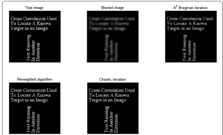
In the first experiment, the images we used were blurred with a ‘disk’ kernel of hsize = . The blurry and restored images are presented in Figure . By comparing these three algo-rithms, it is clear that the reweightedlminimization algorithm performs better in terms of SNR than the chaotic iterative algorithm, and theATBregman iteration lemma is a
lit-tle slower than the chaotic iterative algorithm and theATBregman iteration, which is still acceptable.
In the second experiment the images were blurred with a ‘Gaussian’ kernel of hsize = . The results are shown in Figure . The comparison of the restored effect and the comput-ing time is basically the same as the first one.
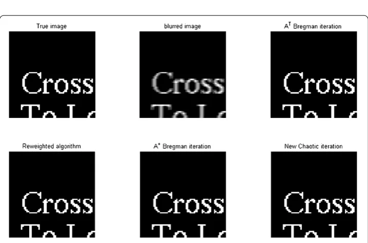
In the third experiment we used a part of the Word image blurred with a × ‘motion’ kernel to better show the local information of the recovered image. The restored small
sparse Word images after using the reweightedl minimization algorithm, the chaotic
iterative algorithm, theAT Bregman iteration, and theA†Bregman iteration are plotted
in Figure . Again we obtain a similar conclusion to the above experiments.
In fact, the complexity analysis also shows comparative results of several methods. Set the same loop number isK. So, the workload of theA†algorithm (.) is two parts. They
[image:8.595.114.478.459.679.2]are the workload of theA†and the loop of the (.). The workload isO(n) during the
Figure 1 Deblurring results of 256×256 sparse Word image convolved by a 15×15 disk kernel generated by the MATLAB command fspecial(‘disk’, 7).Upper left: original image; upper middle: blurred image. The other three are reconstructed images, respectively, by anATBregman iteration, a reweighted
1
Figure 2 Deblurring results of 256×256 sparse Word image convolved by a 7×7 Gaussian kernel generated by the MATLAB command fspecial(‘Gaussian’, 7, 15).Upper left: original image; upper middle: blurred image. The other three are reconstructed images, respectively, by theATBregman iteration, the reweighted1minimization algorithm, and the chaotic iteration.
Figure 3 Deblurring results of 64×80 part of sparse Word image convolved by a 3×5 motion kernel generated by the MATLAB command fspecial(‘motion’, 5, 7).Upper left: original image; upper middle: blurred image. The other four are reconstructed images, respectively, by theATBregman iteration, the reweighted1minimization algorithm, theA†Bregman iteration, and the chaotic iteration.
computation ofA=USV,A†=VTS†UT, whenm<n, because of the singular value
de-composition involving multiplication of the matrix and matrix and eigenvalue calculation. The workload of the loop of the (.) isO(m∗n∗K), because the loop only contains mul-tiplication of matrix and vector. Therefore, the total workload of theA†algorithm (.) isO(n) +O(m∗n∗K). The workload of the chaotic iteration (.), the reweighted l
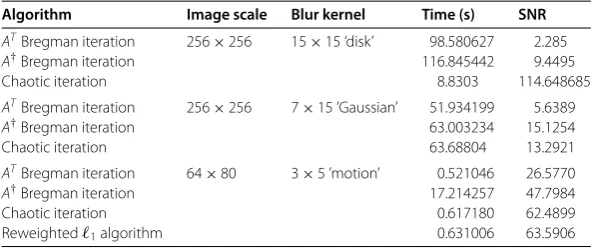
[image:9.595.118.477.358.595.2]Table 1 The comparison of different algorithms
Algorithm Image scale Blur kernel Time (s) SNR
ATBregman iteration 256×256 15×15 ‘disk’ 98.580627 2.285
A†Bregman iteration 116.845442 9.4495
Chaotic iteration 8.8303 114.648685
ATBregman iteration 256×256 7×15 ’Gaussian’ 51.934199 5.6389
A†Bregman iteration 63.003234 15.1254
Chaotic iteration 63.68804 13.2921
ATBregman iteration 64×80 3×5 ’motion’ 0.521046 26.5770
A†Bregman iteration 17.214257 47.7984
Chaotic iteration 0.617180 62.4899
Reweighted1algorithm 0.631006 63.5906
minimization algorithm (.) and theAT Bregman iteration (.) areO(m∗n∗K),
re-spectively. Obviously,K<mn, the workload of theA†algorithm (.) is bigger than
the other three algorithms.
All the experiment data are listed in Table . In summary, for the restored quality of the three methods we have Reweighted > Chaotic >A†AT, while for the computing time the order of magnitude is about : : : . The numerical examples illustrate that the new reweightedlminimization algorithm is fast and efficient for deblurring the image. It is a very useful method.
6 Conclusion
In this paper, we propose the reweightedlminimization algorithm for image deblurring. Above all, we can see that the recovery of the image effect is obvious. Especially in the case of a large degree of blurring and difficult to recover details, it is stable and effective. In addition, we can improve the efficiency of this reweightedlminimization algorithm combining with the ‘kicking’ technology. Because of the scale factor and efficiency of the algorithmA†, the new method proposed in this paper can be used in a parallel operation
to get a better algorithm.
Competing interests
The authors declare that they have no competing interests.
Authors’ contributions
All authors contributed equally to the writing of this paper. All authors read and approved the final manuscript.
Acknowledgements
This research was partly supported by Fund of Oceanic Telemetry Engineering and Technology Research Center, State Oceanic Administration (grant no. 2012003), the NSFC (grant nos. 60971132,61101208) and Fundamental Research Funds for the Central Universities (grant no. 13CX02086A).
Received: 22 February 2013 Accepted: 16 March 2014 Published: 16 June 2014
References
1. Chan, TF, Shen, J: Image Processing and Analysis. SIAM, Philadelphia (2005)
2. Aubert, G, Kornprobst, P: Mathematical Problems in Image Processing, 2nd edn. Appl. Math. Sci., vol. 147. Springer, New York (2006)
3. Andrews, HC, Hunt, BR: Digital Image Restoration. Prentice Hall, Englewood Cliffs (1977)
4. Rudin, L, Osher, S, Fatemi, E: Nonlinear total variation based noise removal algorithms. Physica D60, 259-268 (1992) 5. Dobson, DC, Santosa, F: Recovery of blocky images from noise and blurred data. SIAM J. Appl. Math.56, 1181-1198
(1996)
6. Nikolova, M: Local strong homogeneity of a regularized estimator. SIAM J. Appl. Math.61, 633-658 (2000) 7. Buades, A, Coll, B, Morel, JM: A review of image denoising algorithms, with a new one. Multiscale Model. Simul.4,
490-530 (2005)
9. Buades, A, Coll, B, Morel, JM: Image enhancement by non-local reverse heat equation. CMLA Tech. rep. 22 (2006) 10. Osher, S, Burger, M, Goldfarb, D, Xu, J, Yin, W: An iterative regularization method for total variation-based image
restoration. Multiscale Model. Simul.4, 460-489 (2005)
11. He, L, Marquina, A, Osher, S: Blind deconvolution using TV regularization and Bregman iteration. Int. J. Imaging Syst. Technol.15, 74-83 (2005)
12. Marquina, A: Inverse scale space methods for blind deconvolution. UCLA-CAM-Report 06-36 (2006)
13. Marquina, A, Osher, S: Image super-resolution by TV-regularization and Bregman iteration. J. Sci. Comput.37, 367-382 (2008)
14. Gilboa, G, Osher, S: Nonlocal linear image regularization and supervised segmentation. Multiscale Model. Simul.6, 595-630 (2007)
15. Lou, Y, Zhang, X, Osher, S, Bertozzi, A: Image recovery via nonlocal operators. UCLA-CAM-Report 08-35 (2008) 16. Cofiman, RR, Donoho, DL: Translation-invariant de-noising. In: Antoniadis, A, Oppenheim, G (eds.) Wavelets and
Statistics. Lecture Notes in Statistics, vol. 103. Springer, New York (1995)
17. Hale, E, Yin, W, Zhang, Y: A fixed-point continuation method forl1-regularization with application to compressed sensing. CAAM-TR07-07 (2007)
18. Yin, W, Osher, S, Goldfarb, D, Darbon, J: Bregman iterative algorithms forl1-minimization with applications to compressed sensing. SIAM J. Imaging Sci.1, 143-168 (2008)
19. Cai, J, Osher, S, Shen, Z: Linearized Bregman iterations for compressed sensing. Math. Comput.78(267), 1515-1536 (2009)
20. Cai, J, Osher, S, Shen, Z: Convergence of the linearized Bregman iteration forl1-norm minimization. Math. Comput. 78(268), 2127-2136 (2009)
21. Osher, S, Mao, Y, Dong, B, Yin, W: Fast linearized Bregman iteration for compressive sensing and sparse denoising. UCLA-CAM-Report 08-37 (2008)
22. Cai, J, Osher, S, Shen, Z: Linearized Bregman iterations for frame-based image deblurring. SIAM J. Imaging Sci.2(1), 226-252 (2009)
23. Goldstein, T, Osher, S: The split Bregman method forL1-regularized problems. SIAM J. Imaging Sci.2(2), 323-343 (2009)
24. Cai, J, Osher, S, Shen, Z: Split Bregman method and frame based image restoration. Multiscale Model. Simul.8(2), 337-369 (2009)
25. Wu, C, Tai, X: Augmented Lagrangian method, dual methods, and split Bregman iteration for ROF, vectorial TV, and high order models. SIAM J. Imaging Sci.3(3), 300-339 (2010)
26. Yang, Y, Möller, M, Osher, S: A dual split Bregman method for fastl1minimization. UCLA-CAM-Report 11-57 (2011)
27. Zhang, H, Cheng, L:A–Linearized Bregman iteration algorithm. Math. Numer. Sin.32, 97-104 (2010) (in Chinese)
28. Candés, EJ, Wakin, MB, Boyd, SP: Enhancing sparsity by reweighted1minimization. J. Fourier Anal. Appl.14(5),
877-905 (2008)
29. Wang, G, Wei, Y, Qiao, S: Generalized Inverses: Theory and Computations. Science Press, Beijing (2004) 30. Wang, S, Yang, Z: Generalized Inverse Matrix and Its Applications. Beijing University of Technology Press, Beijing
(1996)
31. Bregman, L: The relaxation method of finding the common points of convex sets and its application to the solution of problems in convex programming. USSR Comput. Math. Math. Phys.7(3), 200-217 (1967)
32. Donoho, D: De-noising by soft-thresholding. IEEE Trans. Inf. Theory41, 613-627 (1995)
33. Schlossmacher, EJ: An iterative technique for absolute deviations curve fitting. J. Am. Stat. Assoc.68, 857-859 (1973) 34. Zhao, YB, Li, D: Reweighted1-minimization for sparse solutions to underdetermined linear systems. SIAM J. Optim.
22(3), 1065-1088 (2012) doi:10.1186/1029-242X-2014-238
Cite this article as:Qiao et al.:A new reweightedl1minimization algorithm for image deblurring.Journal of