Lower bounds for the low rank matrix approximation

R E S E A R C H

Open Access

Lower bounds for the low-rank

matrix approximation

Jicheng Li

_{, Zisheng Liu}

_{and Guo Li}

*_{Correspondence:}

liuzisheng0710@163.com 1_{School of Mathematics and}

Statistics, Xi’an Jiaotong University, No. 28, Xianning West Road, Xi’an, 710049, China

2_{School of Statistics, Henan}

University of Economics and Law, No. 180, Jinshui East Road, Zhengzhou, 450046, China Full list of author information is available at the end of the article

Abstract

Low-rank matrix recovery is an active topic drawing the attention of many

researchers. It addresses the problem of approximating the observed data matrix by an unknown low-rank matrix. Suppose thatAis a low-rank matrix approximation ofD, whereDandAarem×nmatrices. Based on a useful decomposition ofD†–A†, for the unitarily invariant norm · , whenD ≥ AandD ≤ A, two sharp lower bounds ofD–Aare derived respectively. The presented simulations and applications demonstrate our results when the approximation matrixAis low-rank and the perturbation matrix is sparse.

MSC: 15A23; 34D10; 68W25; 90C25; 90C59

Keywords: low-rank matrix; approximation; error estimation; pseudo-inverse; matrix norms

1 Introduction

In mathematics, low-rank approximation is a minimization problem, in which the cost function measures the fit between a given matrix (the data) and an approximating matrix (the optimization variable), subject to a constraint that the approximating matrix has re-duced rank. The problem is used for mathematical modeling and data compression. The rank constraint is related to a constraint on the complexity of a model that fits the data.

Low-rank approximation of a linear operator is ubiquitous in applied mathematics, sci-entific computing, numerical analysis, and a number of other areas. For example, a low-rank matrix could correspond to a low-degree statistical model for a random process (e.g., factor analysis), a low-order realization of a linear system [], or a low-dimensional em-bedding of data in the Euclidean space [], the image and computer vision [–], bioin-formatics, background modeling and face recognition [], latent semantic indexing [, ], machine learning [–] and control []etc. These data may have thousands or even bil-lions of dimensions, and a large number of samples may have the same or similar structure. As we know, the important information lies in some dimensional subspace or low-dimensional manifold, but interfered with some perturbative components (sometimes in-terfered by the sparse component).

LetD∈Rm×n_{be an observed data matrix which is combined as}

D=A+E, ()

whereA∈Rm×n_{is the low-rank component and E∈R}m×n _{is the perturbation}

compo-nent of D. The singular value decomposition (SVD []) is a method for dealing with such high-dimensional data. If the matrixEis small, the classical principal components analysis (PCA [–]) can seek the best rank-restimation ofAby solving the following constrained optimization via SVD of Dand then projecting the columns ofDonto the subspace spanned by therprincipal left singular vectors ofD:

min

E EF

s.t. Rank(A)≤r,

D–AF≤,

()

wherermin(m,n) is the target dimension of the subspace,is an upper bound on the perturbative componentEFand · F is the Frobenius norm.

Despite its many advantages, the traditional PCA suffers from the fact that the estima-tionAˆ obtained by classical PCA can be arbitrarily far from the trueA, whenEis suffi-ciently sparse (relative to the rank ofA). The reason for this poor performance is precisely that the traditional PCA makes sense for Gaussian noise and not for sparse noise. Re-cently, robust PCA (RPCA []) is a family of methods that aims to make PCA robust to large errors and outliers. That is, RPCA is an upgrade of PCA.

There are some reasons for the study of lower bound of a low-rank matrix approximation problem. Firstly, as far as we know, there is no literature to consider the lower bound of the low-rank matrix approximation problem. In our paper, we first put forward the lower bound. Secondly, for the low-rank approximation, when a perturbationEexists, there is an approximation error which cannot be avoided, that is, the approximation error cannot equal , but tends to . Thirdly, from our main results, we can clearly find the influence of the spectral norm ( · ) on the low-rank matrix approximation. For example, for our main result of Case II, when the maximum eigenvalue of the matrixDis larger, the ap-proximation error of (D–A) is smaller. In addition, the lower bound can verify whether the solution obtained by algorithms is optimal. For details, please refer to the experiments Section  of our paper. Therefore, it is necessary and significant to study the lower bound of the low-rank matrix approximation problem.

Remark . PCA and RPCA are methods for the low-rank approximation problem when perturbation item exists. Our aim is to prove that no matter what method is used, the lower bound of error always exists and it cannot be avoided with the perturbation itemE. Considering the existence of error, this paper focuses on the specific situation of this lower bound.

1.1 Notations

For a matrixA∈Rm×n_{, letA}

andA∗denote the spectral norm and the nuclear norm (i.e., the sum of its singular values), respectively. Let·be a unitarily invariant norm. The pseudo-inverse and the conjugate transpose ofAare denoted byA†andAH, respectively. We consider the singular value decomposition (SVD) of a matrixAof rankr

whereU andV arem×randn×rmatrices with orthonormal columns, respectively, andσiis the positive singular values. We always assume that the SVD of a matrix is given

in the reduced form above. Furthermore,A,B =trace(AH_{B) denotes the standard inner}

product, then the Frobenius norm is

AF=A,A =

trAH_{A= m}

i=

n

j=

A_ij 

 =

_r

i= σ_i

  .

1.2 Organization

In this paper, we study a perturbation theory for low-rank matrix approximation. When

D ≥ A orD ≤ A, two sharp lower bounds ofD–Aare derived for a unitarily invariant norm respectively. This work is organized as follows. In Section , we provide a review of relevant linear algebra and some preliminary results. In Section , under dif-ferent norms, two sharp lower bounds ofD–Aare given for the low-rank approximation problem and some proofs of Theorem . are presented. In Section , example and appli-cations are given to verify the provided lower bounds. Finally, we conclude the paper with a short discussion.

2 Preliminaries

In order to prove our main results, we mention the following results for our further dis-cussions.

2.1 Unitarily invariant norm

An important property of a Euclidean space is that shapes and distance do not change under rotation. In particular, for any vectorxand for any unitary matricesU, we have

Ux=x.

An analogous property is shared by the spectral and Frobenius norms: namely, for any unitary matricesUandV, the productUAVH_{is defined by}

UAVH _p=Ap, p= ,F.

These examples suggest the following definition.

Definition .([]) A norm · onCm×n_{is unitarily invariant if it satisfies}

_UAVH _=A

for any unitary matricesUandV. It is normalized if

A=A

Remark . Let=UAVH _{be the singular value decomposition of the matrixAwith}

ordern. Let · be a unitarily invariant norm. SinceUandVare unitary,

A=.

ThusAis a function of the singular values ofA.

The -norm plays a special role in the theory of unitarily invariant norms as the following theorem shows.

Theorem .([]) Let · be a family of unitarily invariant norm.Then

AB ≤ AB ()

and

AB ≤ AB. ()

Moreover,ifRank(A) = ,then

A=A.

We have observed that the spectral and Frobenius norms are unitarily invariant. How-ever, not all norms are unitarily invariant as the following example shows.

Example . Let

A=

   

,

obviously,A∞= , but for a unitary matrix

U=

_

√ 

 √  –√

  √ 

,

we have

UA∞=

_√

  √ 

 

∞ =√

.

Remark . It is easy to verify that the nuclear norm · ∗is a unitarily invariant norm.

2.2 Projection

LetCm_andCn_{bemandn-dimensional inner product spaces over the complex field,}

Definition .([]) The column space (range) ofAis denoted by

R(A) =x∈Cm|x=Ay,y∈Cn ()

and the null space ofAby

N(A) =y∈Cn|Ay= . ()

Further, we let⊥denote the orthogonal complement and getR=N(AH₎⊥ _{andN(A) =}

R(AH₎⊥_.

The following properties [] of the pseudo-inverse are easily established.

Theorem .([]) For any matrix A,the following hold. . IfA∈Cm×n_{has rankn,thenA}†_{= (A}H_A)–_AH_andA†_A=I(n)_. . IfA∈Cm×n_{has rankm,thenA}†_=AH_(AAH₎–_andAA†_=I(m)_.

Here I(n)_∈Rn×n_{is the identity matrix.}

Theorem .([]) For any matrix A, PA=AA†is the orthogonal projector ontoR(A),

PAH=A†A is the orthogonal projector ontoR(AH),I–P_AHis the orthogonal projector onto

N(A).

2.3 The decomposition ofD†_–A†

In this section, we focus on the decomposition ofD†_–A† _{and a general bound of the} perturbation theory for pseudo-inverses. Firstly, according to the orthogonal projection, we can deduce the following lemma.

Lemma . For any matrix A,PA=AA†and PAH=A†A,then we have

P⊥_AA= , AP_A⊥H= , P_A⊥HAH= , A†P⊥A= . ()

Proof SinceP_A⊥=I–PAandP⊥_AH=I–PAH, then we have that

P⊥_AA= (I–PA)A=A–AA†A=A–AAH

AAH–A= ,

AP⊥_AH=A(I–PAH) =A–AA†A=A–A

AHA–AHA= ,

P⊥_AHAH=AH–PAHAH=AH–A†AAH=AH–

AHA–AHAAH= ,

A†P_A⊥=A†(I–PA) =A†–A†AA†=A†–

AHA–AHAA†= .

The proof is completed.

Using Lemma ., the decompositions ofD†–A†are developed by Wedin [].

Theorem .([]) Let D=A+E,then the difference D†_–A†_{is given by the expressions}

D†–A†= –A†ED†–A†P⊥_D+P⊥_AHD†, ()

D†–A†= –A†PAEPDHD†–A†P_AP_D⊥+P⊥

Table 1 Value options forγ

· Arbitrary Spectral Frobenius

γ 3 1+

√

5 2

√ 2

D†_–A†_{= –D}†_P

DEPAHA†+

DHD†P_DHEHP_A⊥

–P⊥_DHEPA

AAH†_{. ()}

By Lemma ., usingPA=AA†,PAH=A†A,P_A⊥=I–P_A,P⊥

AH=I–PAH, these expressions

can be verified.

In previous work [], Wedin developed a general bound of the perturbation theory for pseudo-inverses. Theorem . is based on a useful decomposition ofD†_–A†_{, whereDand} Aarem×nmatrices. Sharp estimates ofD†_–A†_{are derived for a unitarily invariant} norm. In [], Chen et al. presented some new perturbation bounds for the orthogonal projectionsPD–PA.

Theorem .([]) Suppose D=A+E,then the error of D†_–A†_{has the following bound:}

D†–A† ≤γmax A† _, D† _E, ()

whereγ is given in Table.

Remark . For the spectral norm, by formula () we can achieveγ =+ √



 . When·is the Frobenius norm, by formula (), we haveγ =√. Similarly, for an arbitrary unitarily invariant norm, according to formula (), we can deduceγ = .

Remark . From Theorem ., sinceE=D–A, in fact, ifRank(A)≤Rank(D), then () gives the lower bound of the low-rank matrix approximation:

D–A ≥ D

†_–A† γmax{A†

,D†}

. ()

In the following section, based on Theorem ., we provide two lower error bounds of D–Afor a unitarily invariant norm.

3 Our main results

In this section, we consider the lower bound theory for the low-rank matrix approximation based on a useful decomposition ofD†_–A†_{. WhenRank(A)≤Rank(D), some sharp lower} bounds ofD–Aare derived in terms of a unitarily invariant norm. In order to prove our result, some lemmas are listed below.

Lemma .([]) Let D=A+E,the projections PDand PAsatisfy

PDP⊥A=

D†H_P

DHEHP⊥_A=

P⊥_APD H

, ()

therefore

PDP⊥A ≤ D

†

IfRank(A)≤Rank(D),then

P_D⊥PA ≤ PDP⊥A . ()

Lemma .([]) Let A,D∈Cm×n_{, Rank(A) =r,Rank(D) =s,r≤s,then there exists a}

unitary matrix Q∈Cm×m_{such that}

QPAQH= ⎛ ⎜ ⎝

I(r) _{ }      

⎞ ⎟

⎠ and QPDQH= ⎛ ⎜ ⎝



r  rr

 I(s–r) _ rr  r

⎞ ⎟ ⎠, () where r=    I

and r=

   

,

=diag(γ, . . . ,γr), ≤γ≤ · · · ≤γrand=diag(σ, . . . ,σr), ≤σ≤ · · · ≤σr. More-over,γiandσisatisfyγi+σi= ,i= , . . . ,r.

According to Lemma ., we can easily get the following result.

Lemma . Let A,D∈Cm×n_{,Rank(A) =r,Rank(D) =s,r≤s,then we have}

P_A⊥PD = PDP⊥A . ()

Proof Since

P⊥_A=I–PA=QH ⎛ ⎜ ⎝

  

 I(s–r)    I(m–s)

⎞ ⎟

⎠Q, ()

and

PD=QH ⎛ ⎜ ⎝

_r  rr

 I(s–r)  rr  r

⎞ ⎟

⎠Q, ()

then

P⊥_APD=QH ⎛ ⎜ ⎝

  

 I(s–r)  rr  r

⎞ ⎟

⎠Q ()

and

PDP⊥A=QH ⎛ ⎜ ⎝

  rr

 I(s–r) 

  

r ⎞ ⎟

⎠Q. ()

This is a useful lemma that we will use in the proof of the main result. In order to prove our main theorem, two lower bounds ofD–Aare required by the following lemma.

Lemma . For the unitarily invariant norm,ifRank(A)≤Rank(D),then the lower bound of D–A satisfies:

Case I:ForD ≥ A,we have

D–A ≥ D–A– D†–A† DA. ()

Case II:ForD ≤ A,we have

D–A ≥ A–D– D†–A† D_. ()

Proof Case I: SinceD ≥ A, we haveD–A ≥ D–A. Using Theorem . and Lemma ., we haveAB ≤ ABandP⊥DPA ≤ PDPA⊥, respectively. By Lemma .,

we haveP⊥_DD= ,AP_A⊥H=  andA†P⊥A= , this also yields

D–A ≥ D–A=D– PD+PD⊥

PA+P⊥A

A

=D– PDPAA+P⊥DPAA (by Lemma .)

=D–PDPAA– P⊥DPAA byPD⊥P⊥D

≥ D–A– P⊥_DPA A (by Lemma .)

≥ D–A– PDPA⊥ A

=D–A– DD†–A†P⊥_A A

≥ D–A– D†–A† DA (by Theorem .).

Case II: SinceD ≤ A, we haveD–A ≥ A–D. Similarly, by Lemma ., using

P⊥_APD=PDPA⊥, we have

D–A ≥ A–D=A– PA+PA⊥

PD+PD⊥

D

=A– PAPDD+P⊥APDD (by Lemma .)

=A–PAPDD– P⊥APDD byPA⊥P⊥A

≥ A–D– P⊥_APD D

≥ A–D– PDPA⊥ D (by Lemma .)

=A–D– DD†–A†P⊥_A D

≥ A–D– D†–A† D_ (by Theorem .).

We complete the proof of Lemma ..

Our main results can be described as the following theorem.

Case I:ForD ≥ A,we have

D–A ≥ D–A

 +γmax{A†

,D†}DA

. ()

Case II:ForD ≤ A,we have

D–A ≥ A–D

 +γmax{A†

,D†}D

, ()

where the value options forγ are the same as in Table.

Proof Case I: ForD ≥ A, by Theorem . and Lemma . (), we can deduce

D–A ≤ D–A+ D†–A† DA

≤ D–A+γmax A† _, D† _D–ADA,

this yields

D–A ≥ D–A

 +γmax{A†

,D†}DA

. ()

Case II: Similarly, forD ≤ A, by Theorem . and Lemma . (), we can deduce

A–D ≤ D–A+ D†–A† D_

≤ D–A+γmax A† _, D† _D–AD_,

this yields

D–A ≥ A–D

 +γmax{A†

,D†}D

, ()

where the value options forγ are the same as in Table . In summary, we prove the lower

bounds of Theorem ..

Remark . From the main theorem, we can see that ifD=A, thenD–A= . However, in the problem of low-rank matrix approximation,Dis not necessarily equal to A, so the approximation error is present. Furthermore, whenDis close toA, simulations demonstrate that the error has a very small magnitude (see Section ).

4 Experiments

4.1 The singular value thresholding algorithm

Our results are obtained by a singular value thresholding (SVT []) algorithm. This algo-rithm is easy to implement and surprisingly effective both in terms of computational cost and storage requirement when the minimum nuclear norm solution is also the lowest-rank solution. The specific algorithm is described as follows.

For the low-rank matrix approximation problem which is contaminated with perturba-tion itemE, we observe that the data matrixD=A+E. To approximateD, we can solve the convex optimization problem

minA∗

s.t. D–AF≤ε,

()

where · ∗denotes the nuclear norm of a matrix (i.e., the sum of its singular values). For solving (), we introduce the soft-thresholding operatorDτ [] which is defined as

Dτ(A) :=UDτ(S)V∗, Dτ(S) =diag

(σi–τ)+

,

where (σi–τ)+=max{,σi–τ}. In general, this operator can effectively shrink some

sin-gular values toward zero. The following theorem is with respect to the shrinkage operators [–], which will be used at each iteration of the proposed algorithms.

Theorem .([]) For eachτ> and W∈Rm×n,the singular value shrinkage operator Dτ(·)obeys

Dτ(W) =arg min

A τA∗+



A–W 

F,

whereDτ(W) :=UDτ(S)V∗.

By introducing a Lagrange multiplierYto remove the inequality constraint, one has the augmented Lagrangian function of ()

L(A,Y) =A∗–Y,A–D +τ

A–D 

F.

The iterative scheme of the classical augmented Lagrangian multipliers method is

Ak+_{∈arg min}

AL(A,Yk),

Yk+_=Yk_–τ(D–Ak+_). ()

Based on the optimality conditions, () is equivalent to

∈_τ∂(Ak+

∗) +Ak+– (D+τYk),

Algorithm SVT

Task:Approximate the solution of ().

Input:Observation matrixD=A+E, weightτ.Y_=zeros(m,n)

whilethe termination criterion is not met, do Ak+_=D

/τ(D+_τYk), Yk+_=Yk_–τ(D–Ak+_),

k←k+ .

end while Output:A←Ak+_.

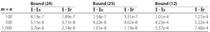
Table 2 Lower bound comparison results

Bound (24) Bound (25) Bound (12)

m = n · 2 · F · 2 · F · 2 · F

100 8.13e-7 1.89e-7 1.54e-7 3.31e-7 1.01e-4 1.27e-4

500 5.11e-8 3.71e-8 4.22e-8 4.62e-8 4.23e-4 5.22e-4

1, 000 3.76e-8 2.14e-8 1.01e-8 1.19e-8 5.57e-4 7.48e-4

where∂(·) denotes the subgradient operator of a convex function. Then, by Theorem . above, we have the iterative solution

Ak+_=D

/τ(D+_τYk),

Yk+=Yk–τ(D–Ak+). ()

The SVT approach works as described in Algorithm .

4.2 Simulations

In this section, we use the SVT algorithm for the low-rank matrix approximation prob-lem. LetD=A+E∈Rm×n_{be the available data. Simply, we restrict our examples to square}

matrices (m=n). We drawAaccording to the independent random matrices and gener-ate the perturbation matrixEto be sparse, which satisfies the i.i.d. Gaussian distribution. Specially, the rank of the matrixAand the sparse entries of the perturbation matrixEare selected to be %mand %m_{, respectively.}

Table  reports the results obtained by lower bounds (), () and (), respectively. Bounds () and () are our new result, bound () is the previous result. Then, com-paring the bounds with each other by numerical experiments, we find that lower bounds (), () are smaller than lower bound ().

4.3 Applications

In this section, we use the SVT algorithm for the low-rank image approximation. From Figures  and , comparing with the original image (a), the low-rank image (b) loses some details. We can hardly get any detailed information from incomplete image (c). However, the output image (d) =Ak_{, which is obtained by the SVT algorithm, can recover the details}

of the low-rank image (b). If we denote image (b) to be a low-rank matrixA, then image (c) is the observed data matrixDwhich is perturbed by a sparse matrixE, that is,

Figure 1 Cameraman. (a)Original 256×256 image with full rank.(b)Original image truncated to be rank 50.(c)50% randomly masked of(b). (d)Recovered image from(c).

Figure 2 Barbara. (a)Original 512×512 image with full rank.(b)Original image truncated to be rank 100.(c)50% randomly masked of(b). (d)Recovered image from(c).

Table 3 Lower bound comparison results of low-rank image approximation

Cameraman Barbara

EF 8.71e-2 7.23e-2

Bound (25) 2.59e-5 1.09e-5

Iters 200 200

5 Conclusion

Low-rank matrix approximation problem is a field which arises in a number of applications in model selection, system identification, complexity theory, and optics. Based on a useful decomposition ofD†_–A†_{, this paper reviewed the previous work and provided two sharp} lower bounds for the low-rank matrices recovery problem with a unitarily invariant norm. From our main Theorem ., we can see that ifD=A, thenD–A= . However, in the problem of low-rank matrix approximation,Dis not necessarily equal toA, so the approximation error is present. Furthermore, from the main results, we can clearly find the influence of the spectral norm ( · ) on the low-rank matrix approximation. For example, in Case II, when the maximum eigenvalue of the matrixDis larger, the error of D–Ais smaller.

Finally, we use the SVT algorithm for the low-rank matrix approximation problem. Ta-ble  shows that our lower bounds (), () are smaller than lower bound (). Simulation results demonstrate that the lower bounds have a very small magnitude. In applications section, we use the SVT algorithm for the low-rank image approximation problem, the lower bounds comparison results are shown in Table . From the comparison results, we find that our lower bounds can verify whether the SVT algorithm can be improved.

Acknowledgements

This work is partially supported by the National Natural Science Foundation of China under grant No. 11671318, and the Fundamental Research Funds for the Central Universities (Xi’an Jiaotong University, Grant No. xkjc2014008).

Competing interests

The authors declare that they have no competing interests.

Authors’ contributions

All authors worked in coordination. All authors carried out the proof, read and approved the final version of the manuscript.

Author details

1_{School of Mathematics and Statistics, Xi’an Jiaotong University, No. 28, Xianning West Road, Xi’an, 710049, China.}

2_{School of Statistics, Henan University of Economics and Law, No. 180, Jinshui East Road, Zhengzhou, 450046, China.}

3_{College of Mathematics and Statistics, Shenzhen University, No. 3688, Nanhai Ave, Shenzhen, 518060, China.}

Publisher’s Note

Springer Nature remains neutral with regard to jurisdictional claims in published maps and institutional affiliations.

Received: 5 August 2017 Accepted: 10 November 2017

References

1. Fazel, M, Hindi, H, Boyd, S: A rank minimization heuristic with application to minimum order system approximation. In: Proceedings of the American Control Conference, vol. 6, pp. 4734-4739 (2002)

2. Linial, N, London, E, Rabinovich, Y: The geometry of graphs and some of its algorithmic applications. Combinatorica

15, 215-245 (1995)

3. Tomasi, C, Kanade, T: Shape and motion from image streams under orthography: a factorization method. Int. J. Comput. Vis.9, 137-154 (1992)

4. Chen, P, Suter, D: Recovering the missing components in a large noisy low-rank matrix: application to SFM. IEEE Trans. Pattern Anal. Mach. Intell.26(8), 1051-1063 (2004)

5. Liu, ZS, Li, JC, Li, G, Bai, JC, Liu, XN: A new model for sparse and low-rank matrix decomposition. J. Appl. Anal. Comput.

2, 600-617 (2017)

6. Wright, J, Ganesh, A, Shankar, R, Yigang, P, Ma, Y: Robust principal component analysis: exact recovery of corrupted low-rank matrices via convex optimization. In: Twenty-Third Annual Conference on Neural Information Processing Systems (NIPS 2009) (2009)

7. Deerwester, S, Dumains, ST, Landauer, T, Furnas, G, Harshman, R: Indexing by latent semantic analysis. J. Am. Soc. Inf. Sci. Technol.41(6), 391-407 (1990)

8. Papadimitriou, C, Raghavan, P, Tamaki, H, Vempala, S: Latent semantic indexing, a probabilistic analysis. J. Comput. Syst. Sci.61(2), 217-235 (2000)

9. Argyriou, A, Evgeniou, T, Pontil, M: Multi-task feature learning. Adv. Neural Inf. Process. Syst.19, 41-48 (2007) 10. Abernethy, J, Bach, F, Evgeniou, T, Vert, JP: Low-rank matrix factorization with attributes. arXiv:cs/0611124 (2006) 11. Amit, Y, Fink, M, Srebro, N, Ullman, S: Uncovering shared structures in multiclass classification. In: Proceedings of the

12. Zhang, HY, Lin, ZC, Zhang, C, Gao, J: Robust latent low rank representation for subspace clustering. Neurocomputing

145, 369-373 (2014)

13. Mesbahi, M, Papavassilopoulos, GP: On the rank minimization problem over a positive semidefinite linear matrix inequality. IEEE Trans. Autom. Control42, 239-243 (1997)

14. Golub, GH, Van Loan, CF: Matrix Computations, 4th edn. Johns Hopkins University Press, Baltimore (2013) 15. Eckart, C, Young, G: The approximation of one matrix by another of lower rank. Psychometrika1(3), 211-218 (1936) 16. Hotelling, H: Analysis of a complex of statistical variables into principal components. J. Educ. Psychol.24(6), 417-520

(1932)

17. Jolliffe, I: Principal Component Analysis. Springer, Berlin (1986)

18. Stewart, GW, Sun, JG: Matrix Perturbation Theory. Academic Press, New York (1990) 19. Wedin, P-Å: Perturbation theory for pseudo-inverses. BIT Numer. Math.13(2), 217-232 (1973)

20. Chen, YM, Chen, XS, Li, W: On perturbation bounds for orthogonal projections. Numer. Algorithms73, 433-444 (2016) 21. Sun, JG: Matrix Perturbation Analysis, 2nd edn. Science Press, Beijing (2001)

22. Cai, J-F, Candès, EJ, Shen, ZW: A singular value thresholding algorithm for matrix completion. SIAM J. Optim.20(4), 1956-1982 (2010)

23. Candès, EJ, Li, X, Ma, Y, Wright, J: Robust principal component analysis? J. ACM58(3), 1-37 (2011)