2018 IX International Conference on Optimization and Applications (OPTIMA 2018) ISBN: 978-1-60595-587-2
On a Linear Control Problem under Interference with a Payoff Depending
on the Modulus of a Linear Function and an Integral
Igor’ IZMEST’EV
1,*and Viktor UKHOBOTOV
1Chelyabinsk State University, Br. Kashirinykh st. 129, 454001 Chelyabinsk, Russia Corresponding author
Control, Interference, Differential game, Electric voltage, Rotor, Lagrange equation.
Abstract. We consider the problem of controlling the rod, which is attached to the rotor of the
electric motor. The control is the value of the voltage applied to the electric motor. The quality criterion is the sum of the angle deviation module that forms the rod with the vertical axis, at a given time, and the integral of the square of the voltage value. We take nonlinear addend in the Lagrange equation of the system as interference. After that, this problem becomes an example of a more general linear control problem under the action of an uncontrolled interference. Applying the results obtained for such problems in the previous works of one of the authors, we construct optimal voltage in the problem of controlling the rod.
Introduction
The linear control problem with an effect of uncontrolled interference and with a fixed termi- nation moment, using a linear change of variables [6], can be reduced to the form when on the right-hand side of the new equations there is only the sum of control and interference whose values belong to given sets depending on the time. In the case that in a linear control problem with interference the payoff is the value of a linear function module at a given moment of time, a linear change of variables leads to a single-type problem when the sets of control and interference values are time-dependent segments. In a more general case, such problems are characterized by the fact that control and interference vectograms are balls whose radii depend on time. Such dynamics after a change of variable arises in well-known differential games “isotropic missiles” [3], control example L.S. Pontryagin [9]. For such differential games, in the case when the terminal set is a ball of a given radius, the form of the alternating integral is found in [9]. In [11], optimal positional strategies for players were constructed. In [12] the form of alternating integral for single-type games with an arbitrary convex closed terminal set is found and optimal positional controls for players are constructed. In work [16], the first player, leading a phase point to a circle of a given radius, minimizes the integral payoff, which is given by the convex function of the norm of his control.
In papers the [13, 14, 15], there are considered the single-type control problems under inter- ference in which control is constructed from the condition of minimization of the payoff, which is the sum of both the terminal and the integral components. In the papers [13, 14], it is assumed that geometric constraints are imposed on the choice of control. In the paper [15], the integral component of the payoff is an integral of the degree of the control value. For these problems,
opti-1
Keywords:
*
mal control existence theorems are proved under rather wide constraints on the class of problems. Necessary and sufficient conditions are found, under which feasible controls are optimal.
Problems on the construction of the law of the voltage supplied to the motor are actual. In [1], such a problem of controlling a pendulum with an electric motor fixed at its end with a flywheel is investigated. In the works [8, 17], a numerical method developed by the authors was applied to solve this problem and computer simulation was carried out.
In our work, we consider the problem of optimal control of the rod, one end of which is rigidly attached to the axis of the electric motor. The Lagrange equation for this system contains a nonlinear addend. Following [2, 18], this added is taken as interference. We obtain a linear control problem in the presence of interference. Applying the results of [15], we construct the optimal voltage for the problem of controlling the rod.
Introductory Example
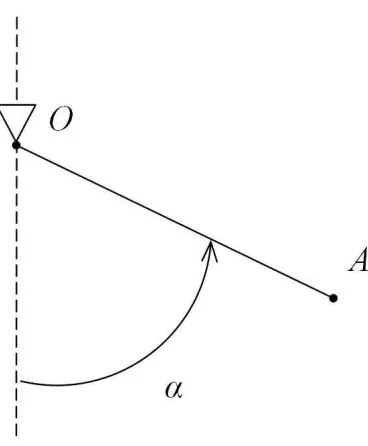
The rotor axis of the electric motor passes through the point O perpendicular to the plane of the figure (see fig. 1). One end of the rodOA is rigidly attached to the axis of the rotor so that it can rotate together with the rotor about its axis in the plane of the figure.
The rotation angle of the rod is denoted by α. The mass of the rod is equal tom. The moment of inertia of a system consisting of the rotor and the rod, with respect to the rotor axis, is denoted byJ.
Neglecting the inductance in the motor rotor circuit, we assume [1, 8, 17] that the moment of electromagnetic forces applied to the rotor on the side of the stator is equal to c1ν−c2α˙, ci >0,
i = 1,2. Here, ν is a voltage applied to the motor. The product c2α˙ describes the moment of
forces, which arise because of counter-emf.
Denote by l the distance from point O to the center of mass of the rod and write down the Lagrange equation, which describes the motion of the system
Jα¨=−mglsinα−c2α˙ +c1ν.
The angle α∗, the time moment p >0 and the weight coefficient f >0 are given. The goal of
choice of applied voltage ν(t) is to minimize value
|α(p)−α∗|f +
Z p
0
ν2(t)dt.
The integral component of the quality criterion determines value of energy consumption. Following [2, 18], we take nonlinear addend in the Lagrange equation as interference
η=−mgl
J sinα.
It is believed that for distance l we know only the estimate of its value 0 < l ≤ l∗. Then for
interference constraint
|η| ≤δ, δ= mgl∗
J
holds. Denote
x1 =α, x2 = ˙α, k =
c2
J, β =
c1
J, ξ = sign ν, φ=|ν|.
Figure 1. The problem of controlling the rod using the rotor of the electric motor.
We assume that sign 0 = 1. Write down the considered problem as a control system under interference
˙
x1
˙
x2
=
0 1 0 −k
x1
x2
+φ
0
β
ξ+
0 1
η, |ξ|= 1, |η| ≤δ
with the quality criterion
|x1(p)−α∗|f+
Z p
0
φ2(t)dt→min
ξ,φ maxη .
Problem statement
We consider the controlled process
˙
x=A(t)x+φB(t)ξ+η, x(t0) =x0; x∈Rn, t ≤p. (1)
Here, p is given termination moment of the control process, and t0 is initial time moment; φ ∈R
and ξ ∈ M are control, and the set M is connected and symmetric with respect to the origin of coordinates compact in Rs; the interference η belongs to the connected compact Q ⊂ Rm; A(t) andB(t) are matrices with corresponding dimensions whose elements are continuous fort0 ≤t≤p
functions.
Let us determine an feasible control. Denote by L2[t0, p] the space of measurable functions
φ: [t0, p]→R with the degreeφ2(r), which is summable on the segment [t0, p]. Feasible control is
non-negative functionφ(·)∈L2[t0, p] and arbitrary functionξ: [t0, p]×Rm →M. The interference
is realized as arbitrary function η: [t0, p]×Rm →Q.
Such a definition of feasible control has the following reason. In the problems of controlling mechanical systems of variable composition, in which the motion is described by the Meshchersky equation [5], a case is possible when the law of variation of the reactive mass must be programmed, and it can be controlled only by the direction of the relative velocity of its separation. In this case, we obtain formulated previously feasible control.
Following [6], the motion of the system (1) generated by feasible control and interference is determined using polygonal lines.
Take the partition ω of the segment [t0, p] with the diameter d(ω)
ω:t0 < t1 < . . . < tj < tj+1 =p, d(ω) = max
i=0,j
(ti+1−ti).
Construct xω(t) fort0 < t≤t1 as solution of Cauchy problem
˙
xω(t) = A(t)xω(t) +φ(t)B(t)ξ(t0, xω(t0)) +η(t0, xω(t0)), xω(t0) =x0.
Denote x1 =xω(t1). Construct xω(t) for t1 < t≤t2 as solution of Cauchy problem
˙
xω(t) = A(t)xω(t) +φ(t)B(t)ξ(t1, xω(t1)) +η(t1, xω(t1)), xω(t1) =x1.
Further, assume that we constructed xω(t) for ti−1 < t≤ti, i≤j. Denote xi =xω(ti). Construct
xω(t) for ti < t≤ti+1 as solution of Cauchy problem
˙
xω(t) = A(t)xω(t) +φ(t)B(t)ξ(ti, xω(ti)) +η(ti, xω(ti)), xω(ti) =xi. (2)
It can be shown that the family of these polygonal lines, which are determined on the segment [t0, p], is uniformly bounded and equicontinuous [11, P. 56]. By Arzela’s theorem [4, P. 104], from
any sequence of the polygonal lines (2) we can select a subsequence that converges uniformly on the segment [t0, p]. The motion of the system (1) realized with feasible φ(t), ξ(t, x), η(t, x) from
the initial state x(t0) = x0 is defined as any uniform limit of the sequence of the polygonal lines
(2), for which diameters of partition d(ω) tend to zero. The quality criterion of control is value
|hψ0, x(p)i −C|f+
Z p
t0
φ2(r)dr. (3)
Here, ψ0 ∈Rm is the given vector, C is the given number; f > 0 is the weight coefficient; h·,·i is
the scalar product inRm.
The control is constructed using the principle of minimization of the guaranteed result [6] of quality criterion (3).
Reduction to One-Dimensional Single-Type Problem
Following [6, P. 160], we pass to a new controlled system, in the equations of motion of which there is no phase vector. Consider fort0 ≤t≤p solutionψ(t) of the Cauchy problem:
˙
ψ =−A∗(t)ψ, ψ(t0) =ψ0. (4)
Here, A∗(t) denotes the transposed of matrix A(t). Denote
b−(t) = min
η∈Qhψ(t), ηi, b+(t) = maxη∈Qhψ(t), ηi. (5)
Then connectivity of compact Q implies [7, P. 33, theorem 4] that
hψ(t), ηi= 1
2(b+(t) +b−(t)) +b(t)v, |v| ≤1, b(t) = 1
2(b+(t)−b−(t))≥0. (6)
Denote
a(t) = max
ξ∈Mhψ(t), B(t)ξi. (7)
Connectivity and symmetry of compact M imply that a(t)≥0 and
hψ(t), B(t)ξi=−a(t)u, |u| ≤1. (8)
Note that functions (5) and (7) are continuous [10, lemma II.3.5]. Hence, the function b(t) in formula (6) is continuous.
Introduce a new variable
z =hψ(t), xi+1 2
Z p
t
(b+(r) +b−(r))dr−C. (9)
Then (4) and (9) imply that z(p) = hψ0, x(p)i −C, and the polygonal line zω(t) corresponding
to the polygonal line (2) is determined by equalities
˙
zω(t) =−φ(t)a(t)ui+b(t)vi, |ui| ≤1, |vi| ≤1.
Thus, we obtain one-dimensional single-type control problem
˙
z =−φ(t)a(t)u+b(t)v, z(t0) =z0; φ(t)≥0, |u| ≤1, |v| ≤1 (10)
with the quality criterion
|z(p)|f+
Z p
t0
φ2(r)dr →min
u maxv . (11)
In this problem, the feasible control is the non-negative function φ(·)∈L2[t0, p] and arbitrary
function u(t, z) with |u(t, z)| ≤ 1. The feasible interference is the arbitrary function v(t, z) with
|v(t, z)| ≤1. The motion z(t) is determined as uniform limit of sequence of the polygonal lines
zω(t) =zω(ti)−
Z t
ti
φ(r)a(r)dr u(ti, zω(ti)) +
Z t
ti
b(r)dr v(ti, zω(ti)),
ti ≤t ≤ti+1, with the diameter of partition d(ω)→0.
Definition 1. The solution of the problem (10), (11) is called the feasible control φ0(t), u0(t, z)
and the number V0 such that
1) for any feasible interference v(t, z) and for any motion z(t) with initial conditionz(t0) = z0,
which corresponds to φ0(t),u0(t, z) and v(t, z), inequality
|z(p)|f +
Z p
t0
φ20(r)dr ≤V0
holds;
2) for any feasible control φ(t), u(t, z) and for any number V < V0 there exists feasible
inter-ference v(t, z) such that for any motion z(t) with initial condition z(t0) = z0 generated by φ(t),
u(t, z) and v(t, z), inequality
|z(p)|f +
Z p
t0
φ2(r)dr > V
holds.
Optimality Conditions in Single-Type Problem
Consider the problem (10), (11) in general case, when z, u,v belongs to the space Rn, and| · |
is the norm in Rn.
Fix a non-negative function φ(·)∈L2[t0, p], a numberε≥0 and consider the differential game
˙
z =−φ(t)a(t)u+b(t)v, |u| ≤1, |v| ≤1 (12)
with the terminal condition
|z(p)| ≤ε. (13)
For the completeness of the exposition we assume that the functions a(t)≥0 and b(t)≥0 are summable on the segment [t0, p] anda(·)∈L2[t0, p].
For such single-type game, L.S. Pontryagin [9] constructed an alternating integral. It follows from its form that the initial position z(t0) belongs to the value of the alternating integral at the
time moment t0 if and only if:
f1(φ(·)) =|z(t0)|+
Z p
t0
(b(r)−φ(r)a(r))dr≤ε, (14)
f2(φ(·)) = max
t0≤t≤p
Z p
t
(b(r)−φ(r)a(r))dr≤ε. (15)
Denote
f(φ(·)) = max(f1(φ(·));f2(φ(·))), (16)
w(z) = z
|z| for |z|>0 and w(0) is any with constraint |w(0)|= 1. (17) Theorem 1 ([11], theorems 8.1 and 8.2).For initial state t0 < p, z(t0) ∈ Rn in the game (12),
(13), the control u = w(z) guarantees the fulfilment of the inequality |z(p)| ≤ f(φ(·)) for any function|v(t, z)| ≤1 and for any realized motion z(t). Control v =w(z) guarantees the fulfilment of the inequality |z(p)| ≥f(φ(·)) for any function |u(t, z)| ≤1 and for any realized motionz(t).
From this theorem, using the formula (16), we obtain that, if the inequalities (14) and (15) hold, then the control u = w(z) guarantees the fulfilment of the inequality (13) for any function
|v(t, z)| ≤1 and for any realized motionz(t). If one of the inequalities (14) and (15) is not satisfied, then the control v = w(z) guarantees the fulfilment of the opposite inequality |z(p)| > ε for any function |u(t, z)| ≤1 and for any realized motion z(t).
Consider the problem
f0(ε, φ(·)) =εf +
Z p
t0
φ2(r)dr →min, (18)
f1(φ(·))≤ε, f2(φ(·))≤ε, ε≥0, φ(·)∈L2[t0, p], φ(t)≥0. (19)
Theorem 2 ([15]).Let us assume that ε0 ≥0 and φ0(t) are a solution of the problem (18), (19).
Then the solution of the problem (10), (11) is the functions φ0(t), u = w(z) and the number
V0 =f0(ε0, φ0(·)).
Theorem 3 ([15]). The solution in the problem (18), (19) exists.
Write down the sufficient conditions for which the number ε0 and the function φ0(t) are the
solution of the problem (18), (19).
Theorem 4 ([15]). Let us assume that the numberε0 and the function φ0 : [t0, p]→R satisfy the
conditions (19). Let there exist a number λ ≥0 and a function θ(t) that is nondecreasing on the segment [t0, p] such thatθ(t0) = 0 and
Z p
t0
θ(r)(b(r)−φ0(r)a(r))dr=θ(p)ε0, (20)
λ
Z p
t0
(b(r)−φ0(r)a(r))dr+|z(t0)| −ε0
= 0, (21)
(f −λ−θ(p))(ε0−ε)≤0 for any ε≥0, (22)
φ0(t) =
a(t)
2 (λ+θ(t)) for t∈[t0, p]. (23) Then the number ε0 and the function φ0(t) are solution of the problem (18), (19).
Theorem 5 ([15]).Let us assume that the conditions of theorem 3 are fulfilled. Then there exists the solution ε0, φ0(t) of the problem (18), (19), for which there exist a number λ ≥ 0 and a
nondecreasing function θ : [t0, p]→R with θ(t0) = 0 which satisfy the conditions (20)–(23).
Example
Write down the system of the differential equations (4)
˙
ψ1
˙
ψ2
=
0 0
−1 k
ψ1
ψ2
, ψ1(p) = 1, ψ2(p) = 0.
The solution of this Cauchy problem is functions
ψ1(t) = 1, ψ2(t) =
1
k 1−e
(t−p)k
Introduce a variable
z =x1+
1
k 1−e
(t−p)k
x2−α∗.
Then
˙
z =−φβ
k 1−e
(t−p)k
u+ δ
k 1−e
(t−p)k
v, u=−ξ, v = 1
δη, |v| ≤1.
Since z(p) = x1(p)−α∗, the quality criterion takes the form
|z(p)|f+
Z p
0
φ2(t)dt →min
u,φ maxv .
For considered problem we obtain
b(t) = δ
k 1−e
(t−p)k
, a(t) = β
k 1−e
(t−p)k
.
Therefore optimality conditions for the problem (18), (19) in considered example take the form
|z(0)|+1
k
Z p
0
1−e(r−p)k(δ−βφ0(r))dr ≤ε0, (24)
1
k 0max≤τ≤p
Z p
τ
1−e(r−p)k(δ−βφ0(r))dr≤ε0, (25)
λ
1
k
Z p
0
1−e(r−p)k(δ−βφ0(r))dr+|z(0)| −ε0
= 0, (26)
1
k
Z p
0
θ(r) 1−e(r−p)k(δ−βφ0(r))dr =θ(p)ε0, (27)
(f −λ−θ(p))(ε0−ε)≤0 for any ε≥0, (28)
φ0(t) =
β
2k 1−e
(p−t)k
(λ+θ(t)). (29)
If ε0 >0, then (28) implies that λ=f −θ(p). Sinceλ≥0 and θ(p)≥0, then 0≤θ(p)≤f.
Take the function θ(r) = 0 for all 0≤r ≤p. Then (27) is satisfied, and the numberλ=f >0. Therefore, (29) implies that
φ0(t) = ψ(t), where ψ(t) =
βf
2k 1−e
(t−p)k
. (30)
Since λ >0, the conditions (24) and (26) become the equality
ε0 =|z(0)|+
1
k
Z p
0
1−e(r−p)k(δ−βψ(r))dr. (31)
Consider the condition (25). Let
δ−βψ(0) ≥0⇔e−kp ≥1− 2kδ
β2f. (32)
Since the functionψ(t) (30) decreases, it follows from the preceding condition and from the equality
φ0(r) = ψ(r) that δ−βφ0(r) > 0 for all 0< r ≤ p. Therefore the maximum value with respect
toτ on the left-hand side of (25) is achieved for τ = 0 and it is positive. Therefore condition (25) follows from the formula (31).
Suppose that the inequality (32) is not satisfied. Since δ−βψ(p) = δ >0,
δ−βψ(r)<0 for 0 ≤r < s and δ−βψ(r)>0 for s < r≤p.
Here, the number
s=p+ 1
k ln
1− 2kδ
β2f
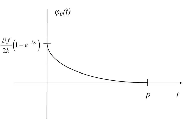
Figure 2. Optimal voltage φ0(t) in the case when either (32) or (33) is satisfied.
is the solution of the equation δ−βψ(s) = 0. In this case, the maximum value with respect to τ
on the left-hand side of (25) is achieved for τ =s, and it is positive. From this and from (31) we obtain that (25) is satisfied if
|z(0)| ≥ 1
k
Z s
0
1−e(r−p)k(βψ(r)−δ)dr. (33)
Thus, if one of the inequalities (32) or (33) is satisfied, then the value of the optimal voltage is determined by the formula (30) (see fig. 2).
Write down one more solution when the inequality (32) is not satisfied and |z(0)|= 0. We take a function θ(r) for which
θ(0) = 0, θ(r) = δf
β
1
ψ(r) for 0< r≤s and θ(r) = f for s≤r ≤p. (34)
Note that this function increases. Then λ= 0. It follows from (29) that
φ0(r) =
δ
β for 0< r≤s and φ0(r) =ψ(r) fors ≤r ≤p. (35)
Substitute the functions (34) and (35) into (27). We obtain
ε0 =
1
k
Z p
s
1−e(r−p)k(δ−βψ(r))dr. (36)
It follows from the equality λ = 0 that the conditions (26) are satisfied. The maximum value respect to τ in (25) is reached when τ =s. Therefore it follows from (36) that inequality (25) is satisfied. Since |z(0)|= 0, the condition (24) is also satisfied.
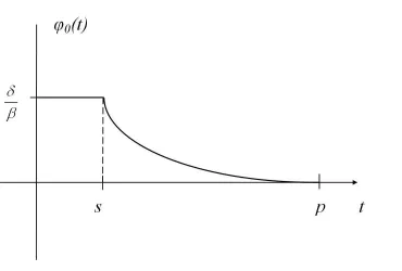
Figure 3. Optimal voltageφ0(t) in the case when (32) is not satisfied, but |z(0)|= 0.
It can be seen from the formula (35) that the value of the optimal voltage at the beginning is constant, and then it decreases (see Fig. 3).
Conclusion
In this paper, we consider the problem of controlling the rod, which is attached to the rotor of the electric motor. The control is the value of the voltage applied to the electric motor. The quality criterion is the sum of the angle deviation module that forms the rod with the vertical axis, at a given time, and the integral of the square of the voltage value. Taking the nonlinear addend in the Lagrange equation of this system as an interference, we obtained a linear control problem with an interference. The resulting linear problem is an example of a more general linear control problem in the presence of interference, in which the payoff consists of two components. The terminal part of the payoff depends on the modulus of a linear function of the phase vector. The integral part of the payoff is the integral on the segment of a degree of scalar function. Applying the results of the paper [15], we construct the optimal voltage for the following cases:
1) the condition (32) is satisfied;
2) the condition (32) is not satisfied, but the condition (33) is fulfilled; 3) the condition (32) is not satisfied, but |z(0)|= 0.
The solution in the remaining cases can be obtained similarly.
Acknowledgements
This research was supported by RFBR (grant no. 18-01-00264 a) and grant of the Foundation for perspective scientific researches of Chelyabinsk State University (2018).
References
[1] A.V. Beznos, A.A. Grishin, A.V. Lenskii, D.E. Okhotsimskii, and A.M. Formal’skii. The control of pendulum using flywheel (in Russian), in: Workshop on Theoretical and Applied Mechanics, Publishing of Moscow State University, Moscow, 2009, pp. 170-195.
[2] F.L. Chernous’ko. Decomposition and synthesis of control in nonlinear dynamical systems, Proceedings of the Steklov Institute of Mathematics. 211 (1995) 414-428.
[3] R. Isaacs. Differential games: A Mathematical Theory with Applications to Warfare and Pursuit, Control and Optimization, John Wiley and Sons, Inc., New York, 1965.
[4] A.N. Kolmogorov and S.V. Fomin. Elements of function theory and functional analysis (in Russian), Nauka Publ., Moscow, 1972.
[5] N.N. Krasovskii. Theory of motion control (in Russian), Nauka Publ., Moscow, 1970.
[6] N.N. Krasovskii and A.I. Subbotin. Positional differential games (in Russian), Nauka Publ., Moscow, 1974.
[7] L.D. Kudryavtsev. A course of mathematical analysis. Vol. 1 (in Russian), Vysshaya shkola Publ., Moscow, 1981.
[8] A.R. Matviychuk, V.I. Ukhobotov, A.V. Ushakov, and V.N. Ushakov. The approach problem of a nonlinear controlled system in a finite time interval, Journal of Applied Mathematics and Mechanics. 81(2) (2017) 114-128.
[9] L.S. Pontryagin. Linear differential games of pursuit. Mathematics of the USSR-Sbornik, Mathematics of the USSR-Sbornik. 40(3) (1981) 285-303.
[10] B.N. Pshenichnyi. Convex analysis and extremum problems (in Russian), Nauka Publ., Moscow, 1980.
[11] V.I. Ukhobotov. Method of one-dimensional design in linear differential games with in-tegral constraints: study guide (in Russian), Publishing of Chelyabinsk State University, Chelyabinsk, Russia, 2005.
[12] V.I. Ukhobotov. The same type of differential games with convex purpose (in Russian), Proceedings of the Institute of Mathematics and Mechanics of the Ural Branch of the Russian Academy of Sciences. 16(5) (2010) 196-204.
[13] V.I. Ukhobotov. A linear control problem under interference with a payoff depending on the modulus of a linear function (in Russian), Proceedings of the Institute of Mathematics and Mechanics of the Ural Branch of the Russian Academy of Sciences. 23(1) (2017) 251-261. [14] V.I. Ukhobotov. Necessary conditions of optimality in linear control problem under
interfer-ence with a payoff depending on the modulus of a linear function (in Russian), Chelyabinsk Physical and Mathematical Journal. 2(1) (2017) 80-87.
[15] V.I. Ukhobotov. On a linear control problem under interference (in Russian), Bulletin of the South Ural State University. Series ”Mathematics. Mechanics. Physics”. 9(2) (2017) 36-46. [16] V.I. Ukhobotov and D.V. Gushchin. Single-type differential games with convex integral payoff,
Proceedings of the Steklov Institute of Mathematics. 275(1) (2011) 178-185.
[17] V.N. Ushakov, V.I. Ukhobotov, A.V. Ushakov, and Parshikov G.V. On solution of control problems for nonlinear systems on finite time interval, IFAC-PapersOnLine. 49(18) (2016) 380-385.
[18] V.I. Vorotnikov and Y.G. Martyshenko. On the nonlinear problem of the three-axis reori-entation of a three-rotor gyrostat in the game noise model, Cosmic Research. 51(5) (2013) 372-378.