On a new semilocal convergence analysis for the Jarratt method

(1)

R E S E A R C H

Open Access

On a new semilocal convergence analysis for

the Jarratt method

Ioannis K Argyros

1

_{, Yeol Je Cho}

2*

_{and Sanjay Kumar Khattri}

3

*_{Correspondence: [email protected]} 2_{Department of Mathematics} Education and the RINS, Gyeongsang National University, Jinju, 660-701, Korea

Full list of author information is available at the end of the article

Abstract

We develop a new semilocal convergence analysis for the Jarratt method. Through our new idea of recurrent functions, we develop new suﬃcient convergence conditions and tighter error bounds. Numerical examples are also provided in this study.

MSC: 65H10; 65G99; 65J15; 47H17; 49M15

Keywords: Jarratt method; Newton-type methods; Banach space; Fréchet-derivative; majorizing sequence; recurrent functions

1 Introduction

In this study, we are concerned with the problem of approximating a locally unique solu-tionx_{of the equation}

F(x) = , (.)

whereF is a Fréchet-diﬀerentiable operator deﬁned on a convex subsetDof a Banach spaceXwith values in a Banach spaceY.

A large number of problems in applied mathematics and also in engineering are solved by finding the solutions of certain equations. For example, dynamic systems are mathemat-ically modeled by difference or differential equations and their solutions usually represent the states of the systems. For the sake of simplicity, assume that a time-invariant system is driven by the equationx˙=Q(x) for some suitable operatorQ, wherexis the state. Then the equilibrium states are determined by solving equation (.). Similar equations are used in the case of discrete systems. The unknowns of engineering equations can be functions (difference, differential and integral equations), vectors (systems of linear or nonlinear al-gebraic equations) or real or complex numbers (single alal-gebraic equations with single un-knowns). Except in special cases, the most commonly used solution methods are iterative - when starting from one or several initial approximations, a sequence is constructed that converges to a solution of the equation. Iteration methods are also applied for solving opti-mization problems. In such cases, the iteration sequences converge to an optimal solution of the problem at hand. Since all of these methods have the same recursive structure, they can be introduced and discussed in a general framework.

Many authors have developed high order methods for generating a sequence approx-imatingx_{. A survey of such results can be found in [, and the references there] (see}

(2)

also [–]). The natural generalization of the Newton method is to apply a multipoint scheme. Suppose that we know the analytic expressions of F(xn),F(xn) andF(xn)–at a recurrent stepxnfor eachn≥. In order to increase the order of convergence and to avoid the computation of the second Fréchet-derivative, we can add one more evaluation ofF(cxn+cyn) orF(cxn+cyn), wherecandcare real constants that are independent

ofxnandyn, whereasynis generated by a Newton-step. A two-point scheme for func-tions of one variable was found and developed by Ostrowski []. Following this idea, we provide a semilocal as well as a local convergence analysis for a fourth-order inverse free Jarratt-type method (JM) [, ] given by

yn=xn–F(xn)–F(xn), Bn=B(n,F) =F(xn)–

F

xn+ 

(yn–xn)

–F(xn)

, (.)

xn+=yn–  Bn

I–

Bn

(yn–xn)

for each n≥. The fourth order of (JM) is the same as that of a two-step Newton method []. But the computational cost is less than that of Newton’s method. In each step, we save one evaluation of the derivative and the computation of one inverse.

Here, we use our new idea of recurrent functions in order to provide new suﬃcient con-vergence conditions, which can be weaker than before []. Using this approach, the error bounds and the example on the distances are improved (see Example . and Remarks .). This new idea can be used on other iterative methods [].

2 Semilocal convergence analysis of (JM)

We present our Theorem . in [] in an aﬃne invariant form sinceF(x)–Fcan be used

forFin the original proof of Theorem ..

Theorem . Let F:D⊆X→Ybe thrice diﬀerentiable.Assume that there exist x∈D, L≥,M≥,N≥andη≥such that

F(x)–∈L(Y,X), (.)

F(x)–F(x)≤η, (.)

F(x)–F(x)≤M, (.)

F(x)–F(x)≤N, (.)

F(x)–

F(x) –F(y)≤Lx–y (.)

for each x,y∈D,

M

 + N M +

L M

 

≤K, (.)

h=Kη≤. (.)

and

Ux,v

=x∈X,x–x ≤v

(3)

where v_{and v}_{are the zeros of functions}

g(t) = K t

_–_t₊_η _(.)

given by

v= – √

 – h

h η, v

= +

√  – h

h η. (.)

Then the following hold:

()The scalar sequences{vn}and{wn}given by

wn=vn–g(vn)–g(vn),

bn=g(vn)–(g(vn+_(wn–vn)) –g(vn)),

vn+=wn–_bn( –_bn)(wn–vn)

⎫ ⎪ ⎪ ⎬ ⎪ ⎪

⎭ (.)

for each n≥are non-decreasing and converge to their common limit v_,_{so that}

vn≤wn≤vn+≤wn+. (.)

()The sequences{xn}and{yn}generated by(JM)are well deﬁned,remain inU(x,v)for all n≥and converge to a unique solution x_∈_U₍_x

,v)of the equation F(x) = ,which is the unique solution of the equation F(x) = in U(x,v).Moreover,the following estimates hold for all n≥:

yn–xn ≤wn–vn, (.)

xn+–yn ≤wn+–vn, (.)

yn–x≤v–wn, (.)

xn–x≤v–vn≤

( –θ)_η₍√

θ)n–

 – √

(



√

θ)n , (.)

where

θ= v

v. (.)

Remarks . The bounds of Theorem . can be improved under the same hypotheses

and computational cost in two cases as follows. Case . Deﬁne a functiongby

g(t) = M

 t

_–_t₊_η_. _(.)

In view of (.), there existsM∈[,M] such that

F(x)–

(4)

for allx∈D. We can ﬁnd upper bounds on the normsF(x)–_F₍_x

)usingM, which is

actually needed, and notKused in []. Note that

M≤K (.)

andK/Mcan be arbitrarily large [–]. Using (.), it follows that, for anyx∈ U(x,v),

F(x)–

F(x) –F(x)≤Mx–x ≤Kx–x ≤Kv< . (.)

It follows from (.) and the Banach lemma on invertible operators [] thatF(x)–_F₍_x )

exists and

F(x)–F(x)≤

  –Mx–x

. (.)

We can use (.) instead of the less precise one used in []:

F(x)–F(x)≤

  –Kx–x

. (.)

This suggests that more precise scalar majorizing sequences{¯vn},{ ¯wn}can be used and they are deﬁned as follows for initial iteratesv¯= ,w¯=η:

¯

wn=v¯n–g(¯vn)–g(v¯n),

¯

bn=b(n,g,g) =g(v¯n)–(g(v¯n+_(w¯n–¯vn)) –g(v¯n)),

¯

vn+=w¯n–_b¯n( –_b¯n)(w¯n–v¯n).

⎫ ⎪ ⎪ ⎬ ⎪ ⎪ ⎭

(.)

A simple induction argument shows that, ifM<K, then

¯

vn<vn, (.)

¯

wn<wn, (.)

¯

wn–v¯n<wn–vn, (.)

¯

vn+–w¯n<vn+–wn (.)

and

¯

v≤v, (.)

where

¯ v= lim

n→∞¯vn.

Note also that ifM=K, thenv¯n=vn,w¯n=wn.

Case . In view of the upper bound forF(xn+)obtained in Theorem . in [] and

(5)

for{xn}and{yn}. Therefore, if they converge under certain conditions (see Lemma .), then we can produce a new semilocal convergence theorem for (JM) with suﬃcient con-vergence conditions or bounds that can be better than the ones of Theorem . (see also Theorem . and Example .).

Similar favorable comparisons (due to (.)) can be made with other iterative methods of the fourth order [, ].

3 Semilocal convergence analysis of (JM) using recurrent functions

We show the semilocal convergence of (JM) using recurrent functions. First, we need the following deﬁnition.

Deﬁnition . LetL≥,M> ,M> ,N≥ andη>  be given constants. Deﬁne the

polynomials on [, +∞) for someα>  by

f(t) = ( +Mη)Mηt+ Mα(α+ )η– α,

g(t) =M( +Mη)t+Mα( +α)

–M( +Mη)]t– Mα,

h(t) =Mη( +α)t+Mη( +α)t+ Mαη

 +

Lη 

+Nαη M +

αMη  – ,

g(t) =Mη( +α)t+

Mα

 +

Lη  +

Nα M +

αM  –Mη

t

–

Mα

 +

Lη

 + Nα

M + αM



.

Moreover, deﬁne a scalarφby

φ=

[Mα_ +_Lη +N__Mαη+αMη_ ]

 –M[η+M(+_Mη)η]

.

The polynomialsf,g,ghave unique positive roots denoted byφf,φgandφg(given in an

explicit form), respectively, by the Descartes rule of signs. Moreover, assume

M

η+M( +Mη)

 η



<  (.)

and

Mα_η

 +

Lη

 + Nαη

M + αMη

 < . (.)

Under the conditions (.), (.), respectively,

φ> ,

(6)

Setφ=min{φh,φf,φg,φg, }. Furthermore, assume

φ≤φ. (.)

Ifφ= , then assume that (.) holds as a strict inequality. From now on (.)-(.)

con-stitute the (C) conditions.

We can show the following result on the majorizing sequences for (JM).

Lemma . Under the(C)conditions,choose

φ∈[φ,φ] ifφ=  and φ∈[φ, ) ifφ= . (.)

Then the scalar sequences{sn},{tn}given by

t= , s=η,

tn+=sn+

M( +M(sn–tn))(sn–tn) ( –Mtn)

,

sn+=tn++

  –Mtn+

M(tn+–sn)

 +

L(sn–tn) 

+NM(sn–tn)



( –Mtn) + M

₍_s

n–tn) ( –Mtn)

(.)

are non-decreasing,bounded from above by

t₌

 + α  –φ

η (.)

and converge to their unique least upper bound t_∈_[,_t_]._Moreover_,_{the following}

esti-mate holds:

≤sn+–tn+≤φ(sn–tn), (.)

where

α=M( +Mη)η

 .

Proof We show, using induction onk, that

≤M( +M(sk–tk))(sk–tk) ( –Mtk)

≤α (.)

and

≤ 

 –Mtn+

Mα

 (sk–tk) + L (sk–tk)

₊NM(sk–tk) ( –Mtk)

+ M

₍_s

k–tk) ( –Mtk)

(7)

The estimate (.) holds fork=  by the choice ofα. Moreover, the estimates (.) and (.) hold forn=  by (.), the choice ofφand (.). Let us assume (.)-(.) hold for

allk≤n. We have in turn by the induction hypotheses:

sk–tk≤φ(sk––tk–)≤ · · · ≤φk(s–t) =φkη,

tk+≤sk+α(sk–tk)≤tk+αφkη+φkη

≤sk–+α(sk––tk–) +αφkη+φkη ≤sk–+αφk–η+αφkη+φkη ≤ · · ·

≤s+αη

 +· · ·+φk+φkη<η+αη( –φ k+₎

 –φ +φ

k_η_,

M(sk–tk) ( –Mtk)

+ M

₍_s

k–tk) ( –Mtk)

≤α

or

 M

M 

(sk–tk) ( –Mtk)

+ (sk–tk)



( –Mtk)

≤ α M,

or

sk–tk  –Mtk

 ≤ α

M

and

NM(sk–tk) ( –Mtk)

=NM( –Mtk)(sk–tk)



( –Mtk)

=NM

 ( –Mtk)

sk–tk  –Mtk



(sk–tk)

≤  M

NM

 (sk–tk)α= Nα

M(sk–tk), M₍_s

k–tk) ( –Mtk)

=M

₍_s

k–tk) 

(sk–tk) ( –Mtk)

≤M  (sk–tk)

α M=

Mα

 (sk–tk).

Hence, instead of (.), we can show

≤ 

( –Mtk+)

Mα

 (sk–tk) + L (sk–tk)

₊Nα

M(sk–tk) +

Mα(sk–tk) 

≤φ. (.)

The estimate (.) can be written as

(8)

or

M +Mφkηφkη≤α+ αM_t_k– Mαtk.

So, we can show, instead of (.),

M +Mφkηφkη+ Mαtk≤α

or

M +Mφkηφkη+ Mα

η+αη

 –φk  –φ

+φk–η

– α≤. (.)

The estimate (.) motivates us to deﬁne polynomialsf¯kon [, ) (forφ=t) by

¯ fk(t) =M

 +Mφkηtkη+ Mαη

 +α

 –tk  –t

+tk–

– α

=Mtkη+Mηtk+ Mα

 +α

 –tk  –t

+tk–

η– α (.)

or, sincet_≤_t_for_t_∈_{[, ], deﬁne the polynomials}_f

kon [, ) by

fk(t) =Mtkη+Mηtk+ Mα

 +α

 –tk  –t

+tk–

η– α. (.)

We need a relationship between two consecutive polynomialsfk:

fk+(t) =Mtk+η+Mηtk++ Mα

 +α

 –tk+

 –t

+tk

η– α+fk(t) –fk(t)

=fk(t) +g(t)tk–η, (.)

wheregand its unique positive rootφg∈[, ) are given in Deﬁnition .. The estimate (.) is true if

fk(φ)≤ (.)

or, if

f(φ)≤, (.)

since by (.) we have

fk(φ) =f(φ). (.)

But (.) is true by the deﬁnition ofφfand (.). Deﬁne

f∞(φ) = lim

(9)

Then we also have

f∞(φ) = lim

k→∞fk(φ) =klim→∞f(φ)≤klim→∞ = . (.) This completes the induction for (.). The estimate (.) is true if

Mα_φk_η

 +

L 

φkη+Nα Mφ

k_η₊αM  φ

k_η_≤_φ_{( –}_M

tk+)

or

Mαφkη

 +

L 

φkη+Nα Mφ

k_η₊αM  φ

k

+φM

 +α

 –φk+  –φ

+φk

η–φ≤. (.)

The estimate (.) motivates us to deﬁne polynomialshkon [, ) by

hk(t) =

Mα  t

k_η₊L η

_tk₊Nα Mt

k_η₊αM  t

k_η

+φM

 +α

 –tk+

 –t

+tk

η–φ. (.)

We need a relationship between two consecutive polynomialshk:

hk+(t) = Mα

 t

k+_η₊L

η

_tk+₊Nα

Mt

k+_η₊αM

 t k+_η

+φM

 +α

 –tk+

 –t

+tk+

η–φ–Mα



 t

k_η_–L η

_tk_–αM  t

k_η

–Nα Mt

k_η_–_φ_M



 +α

 –tk+

 –t

+tk

+φ+hk(t)

and so

fk+(t) =hk(t) +g(t)tkη, (.)

wheregand the unique positive rootφg are given in Deﬁnition .. The estimate (.)

is true if

hk(φ)≤ (.)

or, if

h(φ)≤ (.)

since

(10)

But (.) is true by the deﬁnition ofφhand (.). Deﬁne a functionh∞on [, ) by

h∞(φ) = lim

k→∞hk(φ). (.)

Then we have

h∞(φ) = lim

k→∞hk(φ) =klim→∞h(φ)≤klim→∞ = .

This completes the induction for (.)-(.). It follows that the sequences{sn}and{tn}are non-decreasing, bounded from above byt_{given in a closed form by (.) and converge} to their unique least upper boundt_∈_[,_t_{]. This completes the proof.}

Proposition .[, ] Under the hypotheses of Lemma.,further assume



√

bη< , (.)

where

b=a+M



 and a=

M  +

NM q +

L

. (.)

Fix

q∈



√ b,

η

, η= . (.)

Deﬁne the parameters p,p by

p=_M_( –



√

b q ),

p= Mq

√b, b= ,

⎫ ⎬

⎭ (.)

and a function gon[, /q)by

g(t) =t+

 q +

p q

(qt)

 – (qt) +t 

. (.)

Moreover,assume

mint,g(η)

≤p. (.)

Then the following estimates hold for all k≥:

tk+–sk≤_qp

(qη)k+

,

sk–tk≤_q(qη) k

.

⎫ ⎬

⎭ (.)

Proof We show

(11)

If the estimate (.) holds, then we have

q(sm+–tm+)≤

q(sm–tm)



≤(qη)m+, (.)

which implies the second equation in (.). We have the estimate

M

 (tm+–sm)

₊L

(sm–tm)

₊ NM

( –Mtm)

(sm–tm)+

M

( –Mtm)

(sm–tm)

≤M 

M(sm–tm) ( –Mtm)



+L

(sm–tm)



+ NM

( –Mtm)

(sm–tm)+

M

( –Mtm)

(sm–tm)

≤M 

(sm–tm) ( –Mtm)

+L 

(sm–tm) ( –Mtm)

( –Mtm)

+NM(sm–tm)



( –Mtm)

( –Mtm) +

M



(sm–tm) ( –Mtm)

≤ b(sm–tm) ( –Mtm) ,

that is, we have

sm+–tm+≤

b(sm–tm) ( –Mtm+)( –Mtm)

.

Instead of showing (.), we can show

b(sm–tm)

( –Mtm)( –Mtm+)≤

q(sm–tm) (.)

or

b

( –Mtm+)≤

q, (.)

or

tm+≤p. (.)

By the hypothesis (.), we have

t≤p. (.)

Assume

(12)

We also have

tm+–sm =

M(sm–tm) ( –Mtm)

≤ Mq

√b(sm–tm) ₌_p₍_s

m–tm). (.)

We get in turn

tm+≤(sm–tm) + (tm–sm–) +· · ·+ (t–s) +s+p(sm–tm)

≤η+ q(qη)

m₊_p₍_s

m–tm)+ (sm––tm–)+· · ·+ (s–t)

≤η+ q(qη)

m₊ p q

(qη)(m)+ (qη)(m–)+· · ·+η

=η+ q(qη)

m

+ p q

(qη)

m+

+(qη)

m

+· · ·+(qη) 

+η

≤η+ q+

p q

(qη)(m+)+ (qη)m+· · ·+ (qη)+η

≤η+ q

(qη)

 – (qη)+η 

=g(η)≤p, (.)

which completes the induction for (.). This completes the proof.

Theorem . Under the hypotheses(.)-(.)and(.), further assume that the hy-potheses of Lemma.hold and

Ux,t⊆D. (.)

Then the sequences{xn}and{yn}generated by(JM)are well deﬁned,remain inU(x,t)for

all n≥and converge to a unique solution x_{of the equation F}₍_x_{) = }_in_U₍_x_,_t_)._Moreover_,

the following estimates hold:

yn–xn ≤sn–tn,

xn+–yn ≤tn+–sn,

xn–x≤t–tn,

yn–x≤t–sn.

Furthermore,under the hypotheses of Proposition.,the estimates(.)also hold.Finally, if R≥t_{such that}

U(x,R)⊆D

and

R≤  M

–t,

(13)

Example . LetX=Y=R_,_D_{= [, ]}_,_x

= (, )Tand deﬁne a functionFonDby

F(x) =ξ_– ξ– ,ξ– ξ– 

T .

Using (.)-(.), we obtain

η= ., M= ., N= ., M= ., L= , K= .

and

h= . < ..

Hence the conclusions of Theorem . hold for the equationF(x) = . Considering the hypotheses of Theorem ., from Lemma ., we have

α= .

and, from Deﬁnition ., we get

φf= ., φg= .,

φh= ., φg= ..

Consequently, from the deﬁnition ofφ(see Deﬁnition .), we obtain

φ=φf= .,

and from the deﬁnition ofφ(see Deﬁnition .), we obtain

φ= ..

We see the assumptionφ<φ(see equation (.) in Deﬁnition .) is also valid.

Further-more, from the equation (.) (see Lemma .), we consider

φ= ..

From the equation (.),

t= ..

Hence the conditions of Theorem . are also satisﬁed. Additionally, to verify the claims about the sequences{sn}and{tn}(see equation (.)), we produce Table .

From Table , we observe the following:

The sequences{tn}and{sn}are non-decreasing.

The sequences{tn}and{sn}are bounded from above byt.

(14)

[image:14.595.117.478.99.184.2]

Table 1 The scalar sequences{sn}and{tn}are given by equation (3.5) in Lemma 3.2

n tn sn sn–tn φ(sn–tn)

0 0.000000_×10+00 _1.000000_×₁₀–01 _1.000000_×₁₀–01 _2.000000_×₁₀–02 1 1.106200×10–01 _1.109892_×₁₀–01 _3.691608_×₁₀–04 _7.383216_×₁₀–05 2 1.109893×10–01 _1.109893_×₁₀–01 _9.907814_×₁₀–14 _1.981563_×₁₀–14 3 1.109893×10–01 _1.109893_×₁₀–01 _5.147480_×₁₀–52 _1.029496_×₁₀–52 4 1.109893×10–01 _1.109893_×₁₀–01 _3.750264_×₁₀–205 _7.500528_×₁₀–206 5 1.109893×10–01 _1.109893_×₁₀–01 _1.056649_×₁₀–817 _2.113298_×₁₀–818 6 1.109893×10–01 _1.109893_×₁₀–01 _0.000000_×₁₀+00 _0.000000_×₁₀+00

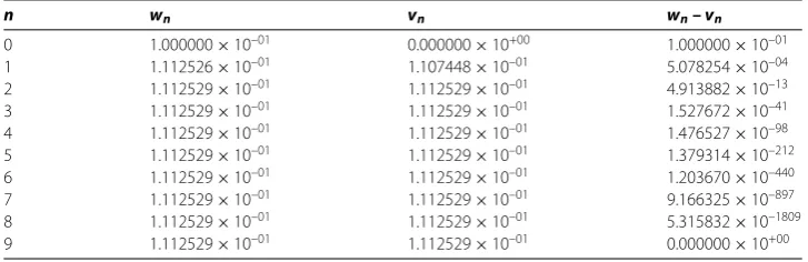
Table 2 The scalar sequences{wn}and{vn}are given by equation (2.11) in Theorem 2.1

n wn vn wn–vn

0 1.000000×10–01 0.000000×10+00 1.000000×10–01 1 1.112526_×10–01 _1.107448_×₁₀–01 _5.078254_×₁₀–04 2 1.112529×10–01 _1.112529_×₁₀–01 _4.913882_×₁₀–13 3 1.112529×10–01 _1.112529_×₁₀–01 _1.527672_×₁₀–41 4 1.112529×10–01 _1.112529_×₁₀–01 _1.476527_×₁₀–98 5 1.112529×10–01 _1.112529_×₁₀–01 _1.379314_×₁₀–212 6 1.112529×10–01 _1.112529_×₁₀–01 _1.203670_×₁₀–440 7 1.112529×10–01 _1.112529_×₁₀–01 _9.166325_×₁₀–897 8 1.112529×10–01 _1.112529_×₁₀–01 _5.315832_×₁₀–1809 9 1.112529×10–01 _1.112529_×₁₀–01 _0.000000_×₁₀+00

Let us now compare the bounds between Theorems . and .. From equation (.), we get

v_{= .}_×_– _and _v_{= .}_×_–_.

From the equation (.), forv[] = , we obtain Table .

Comparing Tables  and , we observe that the bounds of Theorem . are ﬁner than those of Theorem .. That is,sn–tn≤wn–vnfor alln= , , , . . . . Considering the hy-potheses of Proposition ., we have forq= 

a= ., √b= ., p= .,

p= . and g(η) = . <p.

From Table  and the preceding data, we note thatmin{t,g(η)}<p. Consequently, the

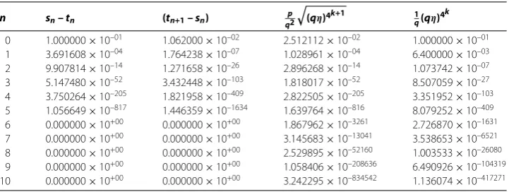
assumption (.) is true. Additionally, to ascertain the estimate (.), we form Table . In Table , we observe that the estimates (.) are also true. Hence the conclusions of Proposition . also hold for the equationF(x) = .

Remarks .[, , ] () The condition (.) can be replaced by a stronger, but easier to check

η

 –δ ≤p, (.)

forδ∈I(see (.) and (.)).

The best possible choice forδseems to beδ=δ. Let

[image:14.595.116.480.218.336.2]

(15)

[image:15.595.118.479.96.232.2]

Table 3 To validate the estimate (3.33) of Proposition 3.3

n sn–tn (tn+1–sn) p

q2

(qη)4k+1 1 q(qη)

4k

0 1.000000×10–01 _1.062000_×₁₀–02 _2.512112_×₁₀–02 _1.000000_×₁₀–01 1 3.691608×10–04 _1.764238_×₁₀–07 _1.028961_×₁₀–04 _6.400000_×₁₀–03 2 9.907814×10–14 _1.271658_×₁₀–26 _2.896268_×₁₀–14 _1.073742_×₁₀–07 3 5.147480×10–52 _3.432448_×₁₀–103 _1.818017_×₁₀–52 _8.507059_×₁₀–27 4 3.750264×10–205 _1.821958_×₁₀–409 _2.822505_×₁₀–205 _3.351952_×₁₀–103 5 1.056649×10–817 _1.446359_×₁₀–1634 _1.639764_×₁₀–816 _8.079252_×₁₀–409 6 0.000000×10+00 _0.000000_×₁₀+00 _1.867962_×₁₀–3261 _2.726870_×₁₀–1631 7 0.000000×10+00 _0.000000_×₁₀+00 _3.145683_×₁₀–13041 _3.538653_×₁₀–6521 8 0.000000×10+00 _0.000000_×₁₀+00 _2.529895_×₁₀–52160 _1.003533_×₁₀–26080 9 0.000000×10+00 0.000000×10+00 1.058406×10–208636 6.490926×10–104319 10 0.000000×10+00 0.000000×10+00 3.242295×10–834542 1.136074×10–417271

In this case, (.) is written as

η≤( –δ)p

 . (.)

() The ratio of convergence ‘qη’ given in Proposition . can be smaller than ‘√θ’ given in Theorem . forqclose to√bandM,N,Lnot all zero andη> .

Setα=√bηandβ=√θ. Note thatb<K and K>b. By comparingα andβ, we have

h=

 K

 –

K b

/

– 

.

Case . If .M_{+ .}_NM_{– .}_L_≤_{ or .}_M_{+ .}_NM_{– .}_L_>

 andη>h, then we have

α<β.

Case . If .M_{+ .}_NM_{– .}_L_{>  and}_η_<_h

, then we have

α>β.

Case . If  <η=h, then we have

α=β.

Note that thep-Jarratt-type method (p∈[, ]) given in [] uses (.)-(.), but the suﬃ-cient convergence conditions are diﬀerent from the ones given in the study and guarantees only third-order convergence (not fourth obtained here) in the case of the Jarratt method (forp= /).

4 Conclusions

(16)

Competing interests

The authors declare that they have no competing interests.

Authors’ contributions

All authors jointly worked on the results and they read and approved the ﬁnal manuscript.

Author details

1_{Department of Mathematical Sciences, Cameron University, Lawton, 73505-6377, Oklahoma.}2_{Department of} Mathematics Education and the RINS, Gyeongsang National University, Jinju, 660-701, Korea.3_{Department of} Engineering, Stord Haugesund University College, Stord, Norway.

Acknowledgements

The second author was supported by the Basic Science Research Program through the National Research Foundation of Korea (NRF) funded by the Ministry of Education, Science and Technology (Grant Number: 2012-0008170).

Received: 29 November 2012 Accepted: 7 April 2013 Published: 22 April 2013 References

1. Argyros, IK: Convergence and Applications of Newton-Type Iterations. Springer, New York (2008)

2. Argyros, IK: On the Newton-Kantorovich hypothesis for solving equations. J. Comput. Appl. Math.169, 315-332 (2004) 3. Argyros, IK: A unifying local-semilocal convergence analysis and applications for two-point Newton-like methods in

Banach space. J. Math. Anal. Appl.298, 374-397 (2004)

4. Argyros, IK, Chen, D, Qian, Q: An inverse-free Jarratt type approximation in a Banach space. Approx. Theory Its Appl. 12, 19-30 (1996)

5. Argyros, IK, Cho, YJ, Hilout, S: Numerical Methods for Equations and Its Applications. CRC Press, New York (2012) 6. Candela, S, Marquina, A: Recurrence relations for rational cubic methods: I. The Halley method. Computing44,

169-184 (1990)

7. Candela, S, Marquina, A: Recurrence relations for rational cubic methods. II. The Chebyshev method. Computing45, 355-367 (1990)

8. Ezquerro, JA, Hernández, MA: Avoiding the computation of the second Fréchet-derivative in the convex acceleration of Newton’s method. J. Comput. Appl. Math.96, 1-12 (1998)

9. Jarratt, P: Multipoint iterative methods for solving certain equations. Comput. J.8, 398-400 (1965/1966) 10. Jarratt, P: Some eﬃcient fourth order multipoint methods for solving equations. Nordisk Tidskr.

Informationsbehandling BIT9, 119-124 (1969)

11. Ostrowski, AM: Solution of Equations in Euclidean and Banach Spaces. Third edition of Solution of equations and systems of equations. Pure and Applied Mathematics, vol. 9. Academic Press, New York (1973)

doi:10.1186/1029-242X-2013-194