http://dx.doi.org/10.4236/ajac.2013.412087
Calculation of the Voigt Function in the Region of Very
Small Values of the Parameter a Where the Calculation Is
Notoriously Difficult
Hssaïne Amamou1, Belkacem Ferhat2, André Bois1
1Laboratoire PROTEE-ISO, Université du Sud Toulon-Var, La Garde, France
2Laboratoire d’Electronique Quantique, Faculty of Physique, University of Sciences and Technology Houari Boumediene,
Alger, Algérie Email: [email protected]
Received September 13, 2013; revised October 25, 2013; accepted November 15, 2013
Copyright © 2013 Hssaïne Amamou etal. This is an open access article distributed under the Creative Commons Attribution License, which permits unrestricted use, distribution, and reproduction in any medium, provided the original work is properly cited.
ABSTRACT
The Voigt function is the convolution of a Lorentzian and a Guaussian density. The computation of these functions is re- quired in several problems arising in a variety of physicochemical subjects; such as nuclear reactors, atmospheric transmit- tance and spectroscopy. In this work we suggest using a new formula for the calculation of the Voigt function. Our for- mula is a new integral representation for the Voigt function that gives the perfect results for the Voigt function calculation and is easily calculable. We give also a comparison between our results of calculation of Voigt function for the very small values of the parameter a, where the calculation is notoriously difficult, with those of the various algorithms of other authors.
Keywords: Convolution; Line Profile; Voigt Function; Lorentz Profile; Doppler Profile and Spectral Lines
1. Introduction
The shape of the spectral lines is a subject of great inter- est in physics and chemistry. Indeed, several important physical and chemical parameters are directly deducted from the spectral lines whose shape is approximated by the Gaussian profile or the Lorentzian profile. Therefore, the parameters obtained do not correspond exactly to the real physical conditions for which the spectral lines have the shape of the distribution of Voigt. For this reason, the study and the calculation of the Voigt function are very interesting in many fields of physics and chemistry. In-deed, for the signal emitted by a plasma, for example, the phenomena that produce the enlargement of the spectral lines are Doppler broadening caused by thermal agitation of the particles, and the enlargement of pressure, which is due to interactions between the transmitters and the neighboring particles, the resulting profile of these phy- sical phenomena is a Voigt profile.
The Voigt function results from the convolution prod- uct between a Gaussian profile and a profile Lorentzian and is expressed by the following formula:
22 2
exp ,
π
x a
V a u x
a u x
02 ln 2
D
u
represents the relationship between
the distance from the center of the Lorentzian line and the width of the Gaussian line.
ln 2 L D
a
determines the importance of Lor-
entzian in the profile, thus if this parameter tends to- wards 0, the Lorentzian is negligible and if it tends to-wards, the infinite the Lorentzian is dominant.
: Frequency.
L
: Lorentz half-width at half maximum in frequency.
D
: Doppler half-width at half maximum in frequency.
0
: Frequency in the center of the line.
This function has been studied recently by several studies [1-8].
2. Calculation of the Voigt Function in the
Region near the u Axis
d (1)
We give our new formula (That we have demonstrated in
the article of Amamou et al. [9] (Demonstration given in
2 2
2 2
0
2 0
2 0
2 π
, exp cos 2 exp
2
π
sin 2 exp exp d
cos 2 cos 2 exp d
sin 2 sin 2 exp d
u
a
a
V a u a au u
au u x x
au ux x x
au ux x x
(2)
This analytical formula of the Voigt function gives a solution to the mathematical problem which is due at the infinite boundaries of the integral which defines the Voigt function. This is a new integral representation for the Voigt function that gives a perfect formula of Voigt func-tion easily calculable and it’s different to the formula given by Roston and Obaid [10] and gives a solution to the problem of exponential growth described by Van Synder [11].
This formula can be used for calculation of the spec-tral lines whose profile is a convolution of a Lorentzian profile and a Gaussian profile. This type of profile de-scribes the actual physical conditions of several phys-icochemical phenomena and its use is very interesting to adjust the spectral lines by theoretical models.
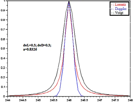
In the Figures 1-3, the determination of the Lorentzian
profile and the Gaussian profile we have used the
fol-lowing parameters; , 0,D,L. These figures shows
the three profiles; Voigt profile, Gaussian profile and
Lorentzian profile for different parameters a and u.
With:
: Wavelength.
L
: Lorentz half-width at half maximum in
wave-length.
D
: Doppler half-width at half maximum in
wave-length.
0
: Wavelength in the center of the line.
In the Figure 1 the Lorentzian profile, the Gaussian
profile and the Voigt profile are given for the following parameters:
0
244 : 0.1: 248 nm, 246 nm,
0.4 nm, 2.3 nm
D L
thus the parameter a4.79.
In the Figure 2 the Lorentzian profile, the Gaussian
profile and the Voigt profile are given for the following parameters:
0
244 : 0.1: 248 nm, 246 nm,
3 nm, 0.003 nm
D L
thus the parameter a0.00083255.
In the Figure 3 the Lorentzian profile, the Gaussian
[image:2.595.78.287.80.192.2]profile and the Voigt profile are given for the following parameters:
[image:2.595.309.540.83.270.2]Figure 1. Voigt profile: “black” Voigt, “blue” Gauss and “red” Lorentz.
Figure 2. Voigt profile: “black” Voigt, “blue” Gauss and “red” Lorentz.
[image:2.595.308.537.311.491.2] [image:2.595.309.537.531.708.2]0
244 : 0.1: 248 nm, 246 nm,
0.3 nm, 0.3 nm
D L
thus the parameter a0.8326.
Our formula is also a very interesting method for easy calculation of the Voigt function. For the calculation of the integrals of Equation (2) the trapezoidal rule method and the adaptive Simpson’s method give very good re- sults.
Table A1 (Appendix 2) gives the values of the Voigt
function calculated with the Formula (2) for the very
small values of the parameter a where the calculation is
[image:3.595.57.286.530.734.2]notoriously difficult [12]. This table gives also the com- putation time(s) for the values of each column of the table. This calculation time depends obviously on the performances of the computer. The computer that we have used has a processor Intel pentium 2.3 GHz and a memory (RAM) 4 GHz. This table gives the reference values of the Voigt function calculated from Equation (2).
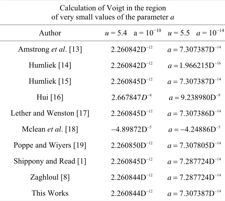
Table 1 gives a comparison between our results of
calculation of Voigt function in the in the region of very
small values of the parameter a with those of the various
algorithms of other authors.
3. Conclusion
The new representation integral for Voigt function that we have demonstrated and used to adjustment “fitting” of lines spectral in a precedent article is used in this work for calculation of Voigt function. Thus, this function is easily calculable. We also made a comparison between the results obtained by our formula and those obtained by the various algorithms of other authors in the region of
Table 1. Comparison between our results and the results of various algorithms of other authors (D is here for 10).
Calculation of Voigt in the region of very small values of the parameter a
Author u = 5.4 a = 10−10 u = 5.5 a = 10−14
Amstrong et al. [13] 2.260842D12 7.307387D14
a
Humliek [14] 2.260842D12 a1.966215D16
Humliek [15] 2.260845D12 7.307387D14
a
Hui [16] 2.667847 8
D a9.238980D9
Lether and Wenston [17] 2.260845D12 a7.307386D14
Mclean et al. [18] 4.89872D5 4.24886D5
a
Poppe and Wiyers [19] 2.260850D12 7.307805D14
a
Shippony and Read [1] 2.260845D12 14 14
7.287724D
a
Zaghloul [8] 2.260844D12 7.287724D
a
This Works 2.260844D12 7.307387D14
a
very small values of the parameter a where the
calcula-tion is notoriously difficult.
REFERENCES
[1] Z. Shippony and W. G. Read, “A Correction to a Highly Accurate Voigt Function Algorithm,” Journal of Quanti-tative Spectroscopy & Radiative Transfer, Vol. 78, No. 2, 2003, pp. 255-255.
http://dx.doi.org/10.1016/S0022-4073(02)00169-3 [2] M. R. Zaghloul and A. N. Ali, “Algorithm 916: Comput-
ing the Faddeyeva and Voigt Functions,” ACM Transac- tions on Mathematical Software, Vol. 38, No. 2, 2011, pp. 1-22. http://dx.doi.org/10.1145/2049673.2049679 [3] J. He and Q. G. Zhang, “An Exact Calculation of the
Voigt Spectral Line Profile in Spectroscopy,” Journal of Optics A: Pure and Applied Optics, Vol. 9, No. 7, 2007, pp. 565-568.
http://dx.doi.org/10.1088/1464-4258/9/7/003
[4] S. M. Abrarov and B. M. Quine, “Efficient Algorithmic Implementation of the Voigt/Complex Error Function Based on Exponential Series Approximation,” Applied Mathematics and Computation, Vol. 218, No. 5, 2011, pp. 1894-1902. http://dx.doi.org/10.1016/j.amc.2011.06.072 [5] F. Schreier, “Optimized Implementations of Rational
Approximations for the Voigt and Complex Error Func- tion,” Journal of Quantitative Spectroscopy and Radia- tive Transfer, Vol. 112, No. 6, 2011, pp. 1010-1025. http://dx.doi.org/10.1016/j.jqsrt.2010.12.010
[6] S. P. Limandri, R. D. Bonetto, H. O. Di Rocco and J. C. Trincavelli, “Fast and Accurate Expression for the Voigt Function. Application to the Determination of Uranium M Linewidths,” Spectrochimica Acta Part B: Atomic Spectroscopy, Vol. 63, No. 9, 2008, pp. 962-967. http://dx.doi.org/10.1016/j.sab.2008.06.001
[7] S. M. Abrarov, B. M. Quine and R. K. Jagpal, “A Simple Interpolating Algorithm for the Rapid and Accurate Cal- culation of the Voigt Function,” Journal of Quantitative Spectroscopy and Radiative Transfer, Vol. 110, No. 6-7, 2009, pp. 376-383.
http://dx.doi.org/10.1016/j.jqsrt.2009.01.003
[8] M. R. Zaghloul, “On the Calculation of the Voigt Line Profile: A Single Proper Integral with a Damped Sine In- tegrand,” Monthly Notices of the Royal Astronomical So- ciety, Vol. 375, No. 3, 2007, pp. 1043-1048.
http://dx.doi.org/10.1111/j.1365-2966.2006.11377.x [9] H. Amamou, A. Bois, M. Grimaldi and R. Redon, “Exact
Analytical Formula for Voigt Function which Results from the Convolution of a Gaussian Profile and a Lor- entzian Profile,” Physical Chemical News PCN, Vol. 43, 2008, pp. 1-6.
[10] G. D. Roston and F. S. Obaid, “Exact Analytical Formula for Voigt Spectral Line Profile,” Journal of Quantitative Spectroscopy & Radiative Transfer, Vol. 94, No. 2, 2005, pp. 255-263. http://dx.doi.org/10.1016/j.jqsrt.2004.09.007 [11] S. Van, “Comment on ‘Exact Analytical Formula for
[12] R. J. Wells, “Rapid Approximation to the Voigt/Faddeeva Function and Its Derivatives,” Journal of Quantitative Spectroscopy and Radiative Transfer, Vol. 62, No. 1, 1999, pp. 29-48.
http://dx.doi.org/10.1016/S0022-4073(97)00231-8 [13] B. H. Armstrong, “Spectrum Line Profiles: The Voigt
Unction,” Journal of Quantitative Spectroscopy and Ra- diative Transfer, Vol. 7, No. 1, 1967, pp. 61-88.
http://dx.doi.org/10.1016/0022-4073(67)90057-X [14] J. Humlicek, “Optimized Computation of the Voigt and
Complex Probability Functions,” Journal of Quantitative Spectroscopy and Radiative Transfer, Vol. 27, No. 4, 1982, pp. 437-444.
http://dx.doi.org/10.1016/0022-4073(82)90078-4 [15] J. Humlicek, “An Efficient Method for Evaluation of the
Complex Probability Function: The Voigt Function and Its Derivatives,” Journal of Quantitative Spectroscopy & Radiative Transfer, Vol. 21, No. 4, 1978, pp. 309-313. http://dx.doi.org/10.1016/0022-4073(79)90062-1
[16] A. K. Hui, B. H. Armstrong and A. A. Wray, “Rapid Computation of the Voigt and Complex Error Functions,”
Journal of Quantitative Spectroscopy & Radiative Trans- fer, Vol. 19, No. 5, 1978, pp. 509-516.
http://dx.doi.org/10.1016/0022-4073(78)90019-5
[17] F. G. Lether and P. R. Wenston, “The Numerical Com- putation of the Voigt Function by a Corrected Midpoint Quadrature Rule for (−∞, ∞),” Journal of Computational and Applied Mathematics, Vol. 34, No. 1, 1991, pp. 75- 92. http://dx.doi.org/10.1016/0377-0427(91)90149-E [18] A. B. McLean, C. E. J. Mitchell and D. M. Swanston,
“Implementation of an Efficient Analytical Approxima- tion to the Voigt Function for Photoemission Lineshape Analysis,” Journal of Electron Spectroscopy and Related Phenomena, Vol. 69, No. 2, 1994, pp. 125-132.
http://dx.doi.org/10.1016/0368-2048(94)02189-7
[19] G. P. M. Poppe and C. M. J. Wijers, “More Efficient Computation of the Complex Error Function,” ACM Transactions on Mathematical Software (TOMS), Vol. 16, No. 1, 1990, pp. 38-46.
http://dx.doi.org/10.1145/77626.77629
Appendix 1
The spectral radiant intensity of Voigt profile is given by:
d I G L G t L t t
(4)With:
2 22 ln 2 4ln 2
exp
π D D
G
(5)
is the Gaussian profile whose D the Doppler half-
width at half maximum and is the frequency.
And
2 20 1 2π 2 L L
L
(6)
is the Lorentzian profile whose L the Lorentz half-
width at half maximum and 0 is the frequency in the
center of the line.
By an adequate change of variables, the convolution Equation (4) can be put in the following form:
ln 2
2
,D
I V a u
(7)
With
2 2 2 exp , d π x aV a u x
a u x
(8)
,V a u is the Voigt function whose parameters are: We can also put the expression (4) in the following form:
2 2 0 1 2 πexp 2π exp π d
4 ln 2
D
L
I
t
i t t
I I
t (9)The two integrals I1
,I2 are given by the following relations:
2 2 0 1 0 2 22 0 0
π
exp 2π exp π d
4 ln 2
π
exp 2π exp π d
4ln 2 D L D L t
I i t t
t
t
I i t t
t (10)which can be also written in the following form:
2 2 0 1 0 2 22 0 0
π π
exp ln 2 exp 2π exp ln 2 d
2 ln 2
π
exp ln 2 exp 2π exp ln 2 d
2 ln 2
L D D D L D D D t L L
I i t
t
t
I i t
t (11)By making the change of variable according to:
0 ln 2 2 ln L D D a u 2 (12)Thus, the preceding relation could be in the following form:
2 0 2 1 0 2 22 0 0
π
exp exp 2π exp d
2 ln 2
π
exp exp 2π exp d
2 ln 2
D
D
t
I a i t a
t
t
I a i t a
By using a suitable change of variable, the expression (13) can be formulated as follows:
2 2
1
2 2
2
2 ln 2
exp exp 2 exp 2 exp d
π
2 ln 2
exp exp 2 exp 2 exp d
π
a D
a D
I a i au iux x x
I a i au iux x x
(14)
Thereafter, we can write the two precedent integrals like:
0 0
2 2
1
2 2
2 0 0
2 ln 2
exp exp 2 exp 2 exp d exp 2 exp d
π
2 ln 2
exp exp 2 exp 2 exp d exp 2 exp d
π
a D
a D
2
2
I a i au iux x x iux x x
I a i au iux x x iux x x
(15)
Thereafter:
2
2
3
0 0
4 ln 2
exp cos 2 cos 2 exp d sin 2 sin 2 exp d
π
D
I a au ux x x au ux x2 x I
(16)with:
2
2
3 0 0
4 ln 2
exp cos 2 cos 2 exp d sin 2 sin 2 exp d
π
a a
D
2
I a au ux x x au ux x
x (17)By a relatively simple mathematical analysis we can give the following solutions:
2 4
2 2
0 0
3
2 2
0 0 0
2 2 π
cos 2 exp d 1 exp d exp
1.2 1.2.3.4 2
2
sin 2 exp d 2 exp d exp exp d
1.2.3
u
ux ux
ux x x x x u
ux
ux x x ux x x u x x
2
2 2
(18)
Thus, the Voigt profile can be written in the following form:
2
2
2
2
3 0
4 ln 2 π
exp cos 2 exp sin 2 exp exp d
π 2
u
D
I a au u au u x x I
(19)From this manner and according to the Equation (7) we express the Voigt function in the following way:
2 2 2
0
2 2
0 0
π
, exp cos 2 exp sin 2 exp exp d
2
cos 2 cos 2 exp d sin 2 sin 2 exp d
u
a a
V a u a au u au u x x
au ux x x au ux x x
2
Appendix 2
Tab
le A1. Cal
cu
lation
of Voigt
fu
n
ction
very
s
m
all va
lu
es
of t
h
e p
a
ramete
r
a
. We g
ive also th
e ca
lculation
times of
each
12
values of ea