Real Time Data Revisions and the PCE Measure of Inflation

Munich Personal RePEc Archive

Real-Time Data Revisions and the PCE

Measure of Inflation

Tierney, Heather L.R.

College of Charleston

February 2010

Real-Time Data Revisions and the PCE Measure of Inflation

By

Heather L.R. Tierney

April 2010

Abstract

This paper tracks data revisions in the Personal Consumption Expenditure using the exclusions-from-core inflation persistence model. Keeping the number of observations the same, the regression parameters of earlier vintages of real-time data, beginning with vintage 1996:Q1, are tested for coincidence against the regression parameters of the last vintage of real-time data, used in this paper, which is vintage 2008:Q2 in a parametric and two nonparametric frameworks. The effects of data revisions are not detectable in the vast majority of cases in the parametric model, but the flexibility of the two nonparametric models is able to utilize the data revisions.

KEY WORDS: Inflation Persistence, Real-Time Data, Monetary Policy, Nonparametrics, In-Sample Forecasting

JEL Classification Codes: E52, C14 , C53

∗

Contact Author: Heather L.R. Tierney, School of Business and Economics, College of Charleston; 5 Liberty Street, Charleston, SC 29424, email: tierneyh@cofc.edu; phone: (843) 953-7070; fax: (843) 953-5697. I would like to thank in alphabetical order the following people for their gracious comments: Marcelle Chauvet, Zeynep Senyuz, Mototsugu Shintani, Tara Sinclair, Emre Yoldas, and last but not least, the participants of the 17th _{Annual Symposium of the Society for Nonlinear Dynamics and Econometrics (2009). I also give a special}

1.

Introduction

Real-time data gives the researcher access to the lastest available information that

can be used in policy analysis. The general train of thought is: the more information, the

better. This would hold true, especially, if the information is being utilized. According to

Croushore and Stark (2001), the revisions in real-time data are typically just a few tenths,

but these small changes can be gleaned and applied if the appropriate economometric tool

is used such as a flexible nonparametric model, which this paper employs.

The data revisions can come from two sources: the updating of previously released

data and benchmark revisions. The updating of previously released datum can occur up to

three years after the initial release and occurs when new information becomes available or

an error in calculating the original statistic is remedied. Benchmark revisions occur every

five years and could possibly include new data from economic censuses as well as possible

methodological changes such as the switch to the chain-weighted GDP, which occurred in

1996.1

In regards to using quarterly data, which this paper analyzes, a maximum of twelve

observations of a given real-time data set has the potential of changing at any given time,

aside from the benchmark revisions. As stated by Croushore and Stark (2003), generally

not all of the potential twelve observations change simultaneously.

Since 2007, the Federal Reserve has been using both total and core Personal

Consumption Expenditure (PCE) for forecasting inflation due to one reason being that both

time series are subject to revision (Croushore 2008).2 _{Regarding previous work on the}

effects of data revisions and the PCE, Croushore (2008) analyzes the changes in the

magnitudes and the pattern of the data revisions of PCE. This paper tracks real-time data

revisions in PCE in the exclusions-from-core model of inflation persistence of Lafléche and

Armour (2006) and Tierney (2009), which are based upon Cogley (2002). The purpose is

to see if the data revisions, which are generally small in magnitude, have an impact on the

parameters of the exclusions-from-core inflation persistence model by producing

statistically different parameters, which might be of future use in policy analysis.

1 _{Please see Croushore and Stark (2001) and Croushore (2007) for more information regarding the data}

collection methods of the real-time dataset.

Tierney (2009) finds that the effects of data revisions are difficult to determine

when a recursive framework is implemented since both new data as well as revised data is

used in a new vintage, i.e. real-time dataset.3 _{The estimated parameters of a model are}

changing, but it is difficult to determine, with any degree of certainty, whether the changes

are coming from the newly incorporated data or the revised data. In this paper, instead of

using just one particular vintage or one particular revision for tracking the effects of data

revisions, all available vintages and all available revisions are able to be examined

simultaneously as has been suggested by Elliott (2002).

In regards to denoting the vintages, each vintage will have the prefix of “V_” in order

to distinguish it from a given observation. For instance, V_1996:Q1, which is the first

available vintage of PCE, refers to the vintage of the real-time dataset released in the

middle of the first quarter of 1996 with the data ranging being from 1983:Q4 to 1995:Q4

for this paper. The sample size increases by an increment of one with each additional

vintage. The last vintage of real-time PCE used in this paper is V_2008:Q2 with the data

ranging from 1983:Q4 to 2008:Q1.

To test for the effects of data revisions, each earlier vintage is tested against

V_2008:Q2, while keeping the number of observations the same in each comparison. The

regressions produced by the two separate vintages are then tested for coincidence. This

translates into testing whether the estimated intercepts and slope coefficients are

statistically equivalent between the two comparison vintages at the 5% significance level.

If this is the case, then data revisions are too small to be detected and hence are not useful

for implementation in policy matters in the given methodology.

Three different methodologies are used to test for coincidence. Lafléche and

Armour’s (2006) model of Ordinary Least Squares (OLS) is used as a benchmark

comparison against two versions of the kernel weighted least squares (KWLS) method of

nonparametrics.4 _{The first nonparametric methodology involves using the average of all}

the local conditional nonparametric estimators, which is referred to as the global

3 _{For a summary of the uses of real-time data, please see Croushore and Stark (2001) and (2003).}

4 _{The KWLS nonparametric model is also known as the Local Linear least Squares (LLLS) nonparametric}

nonparametric model. It is offered as a measure of central tendency and is meant as a

direct comparison against OLS.

The second methodology involves using the local results of the nonparametric

regression produced conditional on just the very last observation, i.e. the Tth_{observation of}

each comparison vintage. As it pertains to policy, examining just the Tth _{local conditional}

regression is a very useful tool because it utilizes the latest available information while

automatically incorporating the information in the relevant time-frame through the use of

KWLS. For instance, in deciding whether to raise or lower interest rates in response to

inflation, the Federal Reserve might look at historical periods that contain inflation similar

to the current level of inflation. The Tth _{local conditional regression automatically}

incorporates related periods by placing a higher weight on observations closer to the Tth

conditioning observation within the window width.5

In regards to real-time data, with only a few observations changing by a small

magnitude at a given time, this paper finds that an econometric model that is

aggregate-driven such as OLS is unable to utilize the subtlety of the new information, while both

versions of the KWLS nonparametric model is able to do so especially at the Tth _local

conditional level. Thus, data revisions do have an impact on the exclusions-from-core

measures of inflation over a five-period in-sample forecast horizon of one, two, four, eight,

and twelve quarters given the proper econometric tool.

The structure of this paper is of the following format: Section II presents the

theoretical methodologies. A brief discussion of the univariate data and the empirical

results are presented in Section III. The conclusion is presented in Section IV.

2.

Theoretical Methodologies

Before the effects of data revision of core and total inflation can be examined, a

discussion of the exclusions-from-core inflation persistence model is necessary. The

exclusions-from-core inflation persistence model is used in both the parametric and

nonparametric case and is discussed without a loss of generality with respect to only one

5 _{For more information on the nonparametric exclusions-from-core inflation persistence model, please see}

vintage, i.e. real-time dataset.6 _{For both the parametric and nonparametric models, the}

regressand, Yt =

(

)

regressor,

(

)

t t t

X = π −π , is the difference between core inflation and total inflation at time t, which is the exclusions-from-core measure of inflation. For the calculation of

inflation, the PCE is used for both core and total inflation. Regarding the testing for the

effects of data revisions, this is accomplished by testing for coincidence by examining the

same sample period in two comparison vintages at a time in a given in-sample forecast

horizon.

2.1 The Parametric and Nonparametric Inflation Persistence Models

Both the parametric and nonparametric methodologies model the conditional mean

of m

( )

(

)

(

)

{

(

)

}

1

, T ,

t t _t

X Y

= in

the following regression function:

( )

t t t

Y =m X +ε . (1)

Regarding the parametric model, the conditional mean is denoted as

( )

( )

m X =m X with the subscript p referring to the parametric regression. The OLS regression model is of the following forms:

( )

t p t t

Y =m X +u (2)

t t t

Y =α+βX +u , (3)

with

(

)

0,

t t

u σ and where mp

( )

one set of regression parameters is produced.

One of the main benefits of using the exclusions-from-core inflation persistence

model is that it permits the study of inflation persistence in a stationary framework.7 _One

problem in using the afore-mentioned model is autocorrelation, which is addressed

through the use of the Newey-West (1987) heteroskedasticity and autocorrelation

6 _{For more details on the exclusions-from-core examination of inflation persistence, please see Johnson}

(1999), Clark (2001), Cogley (2002), Rich and Steindel (2005), Lafléche and Armour (2006), Tierney (2009).

7 _{For more information regarding the stationarity of the exclusions-from-core-inflation persistence model,}

consistent (HAC) covariance matrix in the parametric and nonparametric model as has

been implemented by Cogley (2002), Rich and Steindel (2005), and Tierney (2009). The

Newey-West (1987) HAC covariance matrix is used to form the standard errors and the

t-statistics for the exclusions-from-core inflation persistence model with the lags of the

Bartlett kernel reflecting the length of the h-period in-sample forecast horizons.8

Similarly for the nonparametric regression, the conditional mean is denoted as

( )

( )

m X =m X , with the subscript np referring to the nonparametric regression. For any

given x and for

(

( )

)

0,

t x

υ σ , the KWLS nonparametric model, which produces T sets of

time-varying regression parameters, is:

( )

t np t t

Y =m X +υ (4)

( )

( )

t t t

Y =α x +β x X +υ (5)

with m_np

( )

( )

( )

The KWLS nonparametric model differs from the parametric model in its flexibility,

which enables the small changes of data revisions to be more readily incorporated and

utilized. The flexibility as well as the minmax properties of the KWLS regression model

comes from fitting a line within a certain bandwidth, i.e. window width conditional on each

and every observation, x in the dataset, which helps to balance the bias-variance trade-off

and produce T-sets of time-varying coefficients.9

In addition, the KWLS nonparametric regression model provides an adaptive

learning framework through the use of the window width. It is able to automatically

incorporate new data based on relevance in relation to the conditioning observation for

each and every single x. In regards to the incorporation of data revisions, this flexibility

permits the gleaning of new, small-in-magnitude information, which can be lost in an

aggregate-driven model such at the OLS.

8 _{Regarding the estimation of the Newey-West HAC variance-covariance matrix, the procedure written by}

Mika Vaihekoski (1998, 2004) is used and is able to be obtained from the following web address: http://www2.lut.fi/~vaihekos/mv_econ.html#e3.

9 _{For more information regarding the nonparametric methodology, please refer to Ruppert and Wand (1994),}

A set of global nonparametric regression parameters are formed by taking the

average of all the local conditional nonparametric regression parameters of Equation (5).

This permits one to compare the averaged OLS parameters with a set of averaged

nonparametric parameters.

For this paper, conditional on any given x, the univariate Gaussian kernel is used as

the smoothing, i.e. weighting function, which is of the form:

( )

T

t 1

K K ψ

=

= , (6)

where

_{( )}

(

)

= − with t

T

x x d

ψ = − and dT referring to the window

width, which is the smoothing parameter of the model. Within the realm of the window

width, the closer any given x_{t is to the conditioning observation,} x, the higher the weight and vice versa.

The flexibility provided by nonparametrics is due to its window width, and it is also

its weakness since the choice of window width can severely affect the estimation of the

local conditional regression parameters.10 _{For this paper, the pre-asymptotic, data-driven}

residual-based window width approach of Fan and Gijbels (1995), which is the integrated

residual squares criterion (IRSC) method, is used to obtain the window width. As

previously noted by Fan and Gijbels (1995), Marron (1988), and Härdle and Tsybakov

(1997), the use of the IRSC also minimizes the squared bias and the variance of the

regression parameters, which provides a constant window width for each dataset, but it is

not constant across the fifty vintages of real-time data.11

Robinson (1998) notes that the nonparametric methodology takes into account

heteroskedasticity but not autocorrelation. Even though the parameters are not affected,

autocorrelation needs to be addressed since it produces standard errors that could be

underestimated. This would then produce test statistics that are overestimated. Härdle,

Lütkepohl, and Chen (1997) state that the principle of ‘whitening by window width’ does

10 _{The Curse of Dimensionality is a non-issue since a univariate model is used in this paper (Cleveland and}

Devlin 1988, Härdle and Linton 1994).

11 _{For other papers that use the residual-based window, please see Cai (2007), Cai and Chen (2006), Cai, Fan,}

not apply since it pertains to removing autocorrelation within the window width only.

Hence, due to the formation of the leading variables used in the nonparametric regressions,

the Newey-West (1987) HAC covariance matrix is needed to removed the autocorrelation.

and to form the standard errors and the test statistics.12

The parametric OLS model of inflation persistence using the exclusions-from-core

measure of inflation of Equation (3) is of the following form:

(

)

(

)

t h t t t ut

π ₊ −π =α+β π −π + (7)

where πt h+ is the h-period-ahead total inflation at time t, πt is total inflation at time t, _t core

π

is core inflation at time t,

( )

(

)

p t t t

m X =α+β π −π , and

(

)

~ ,

t t

u oσ being the distribution

of the random error term, ut with h representing the in-sample forecast horizon.13

The KWLS nonparametric regression model of inflation persistence using the

exclusions-from-core measure of inflation of Equation (3) is of the following form:

(

)

( )

( )

(

)

t h t x x t t t

π₊ −π =α +β π −π +υ (8)

where core

x=π −π and

( )

( )

( )

(

)

np t t t

m X =α x +β x π −π . Equation (8) is calculated conditional on each and every single observation of the regressor in the dataset thereby

producing a total of T local conditional nonparametric regressions. In regards to the local

analysis, only the Tth _{local conditional nonparametric regression of Equation (8) is used.}

2.2 Testing for the Effects of Data Revisions

The general idea for testing for the effects of data revisions necessitates analyzing

the same sample period in the three previously mentioned methodologies and to testing for

coincidence. As noted by Kleinbaum and Kupper (1978) and Howell (2007), when two

regressions have coincidence, in this case, this means that the intercepts and slopes

produced by the two comparison vintages, Vintages K and L are statistically equivalent.

Vintage K ranges from {V_1996:Q1, V_1996:Q2, …, V_2008:Q2}, and Vintage L refers to the

very last vintage examined in this paper, which is V_2008:Q2.

12 _{For more on the use of the Newey-West HAC covariance matrix in the parametric methodology, please see}

Cogley (2002) and Rich and Steindel (2005), and for the nonparametric methodology, please see Tierney (2009). For the use of the t-statistic in nonparametrics, please see Wasserman (2006).

13 _{For more information regarding the interpretation of the exclusions-from-core-inflation persistence model,}

The parametric OLS model of inflation persistence using the exclusions-from-core

measure of inflation of Equations (7) is used to explain the test for coincidence. In the

parametric model, the regression coefficients from the regression from Vintages K and L

are compared and are denoted respectively as the following:

(

)

(

)

Kt h Kt K K Kt Kt uKt

π ₊ −π =α +β π −π + (9)

and

(

)

(

)

Lt h Lt L L Lt Lt uLt

π ₊ −π =α +β π −π + (10)

The hypothesis test of the parametric regression for coincidence is of the following form:

Ho: αK =αL and βK =βL (Regressions have coincidence)

versus

H1: α_K ≠α_L or β_K ≠β_L (Regressions do not have coincidence) (11)

A t-statistic using a pooled variance term, assuming dependence, that takes into

account autocorrelation within each dataset as well as the correlation between Vintages K

and L is used to separately compare the intercepts and slopes of Vintages K and L. Since a

pooled variance is utilized, the question of which degrees of freedom (df) to use in the

calculation of the critical value arises. To determine the df, an F-test at the 5% significance

level comparing the unconditional variance of the error terms of Vintage K and Vintage L is

used and is as follows:

Ho: σ_L2 =σ_K2 versus H1: σ_L2 ≠σ_K2 (12)

as noted by Kleinbaum and Kupper (1978) and Howell (2007). If the null fails to be

rejected then the df for the t-test becomes:

L K

df =T +T −2. (13)

If the null is rejected, then the df for the t-test becomes:

L

df =T −1 or df =TK −1.

Since the total number of observations, which is denoted as TK and TL for Vintages K and L

respectively, are the same, then TL = TK.

Assuming dependence, the t-test for both the intercept and the slopes are of the

(

)

(

(

)

)

2 2

L K

t_α = α −α σ_α +σ_α −2*ρσ σ_{α α} (15)

and

(

)

(

(

)

)

L K L K

2 2

L K

t_β = β −β σ_β +σ_β −2*ρσ σ_{β β} (16)

where ρ refers to the covariance of the error terms of the regressions of Vintage K and

Vintage L. The Newey-West (1987) standard errors of the intercepts of Vintages K and L

are

K

α

σ and

L

α

σ respectively, and the Newey-West (1987) standard errors of the slope

coefficients of Vintages K and L are

K

β

σ and

L

β

σ . In the case of assuming correlated data, the df is that of Equation (14) and is confirmed by rejecting the null of equal variances. The

covariance of the error terms is used since many observations are identical in each of the

comparisons of Vintages K and L since only a maximum of twelve observations of a given

dataset can change due to data revisions with the exclusion of the benchmark years.

In regards to analyzing the effects of data revisions from V_1996:Q1 to V_2008:Q2, a

recursive methodology that keeps the same sample size for Vintages K and L with the

sample size being that of Vintage K is as follows:

(i.) The OLS parameters from Equations (7) and the global nonparametric

parameters, which is the average of all the TK and TL nonparametric

parameters for Vintages K and L from Equation (8) are obtained for each of

the two vintages and tested for coincidence within each respective

methodology. Regarding the local nonparametric model, only the TKth local

conditional KWLS nonparametric parameters from Vintage K and the TLth

local conditional KWLS nonparametric parameters from Vintage L of

Equation (8) are tested for coincidence. This will be done for all five

in-sample forecast horizons since the updating of data can occur for a maximum

of three years excluding the benchmark revisions.

(ii.) Repeating Item (i.) with Vintages ( K +1 ) and L, the OLS, global

nonparametric, and the local nonparametric regression parameters

conditional on ₍th ₎ K 1

T ₊ and ₍th ₎ L 1

T ₊ are again obtained and are tested for

(iii.) This iterative method is done for all remaining vintages while holding each of

the observations and in-sample forecast horizons constant for each dataset

until Vintage K equals Vintage L.

Testing the Tth _{local conditional nonparametric regression model and the global}

nonparametric model for coincidence is analogous to the testing of the parametric model.

Using the parameters from the Tth _{local conditional nonparametric regression model from}

Equation (8), the hypothesis test for the Tth _{local conditional nonparametric regression}

model for coincidence is of the following form:

Ho:

( )

( )

K L

T T

x x

α =α and

( )

( )

K L

T T

x x

β =β

versus

H1:

( )

( )

K L

T T

x x

α ≠α or

( )

( )

K L

T T

x x

β ≠β . (17)

The hypothesis test of Equation (17) is of particular interest because it directly

compares the last observation of Vintage K with its counter-part in Vintage L, which is the

observation that is most likely to be updated. This permits one to see if the parameters of

the Tth _{local conditional nonparametric regression model are affected by data revisions.}

The t-test is analogous to that of Equations (15) and (16) except for using the Newey-West

(1987) standard errors of the intercepts and slope coefficients of Vintages K and L that are

obtained from the Tth _{local conditional nonparametric regression from each comparison}

vintage.

Regarding the test for coincidence of the global nonparametric model, the average of

all the local conditional nonparametric parameters is used to form the hypothesis test of

Equation (17) instead of using just the Tth _{local conditional nonparametric regression}

parameters. The Newey-West (1987) standard errors from all the T local nonparametric

regressions are used to form the t-statistic for the global nonparametric regression model

since these residuals are obtained my minimizing the sum of squared errors. Lastly, the

t-test is formed in the same manner as that of Equations (15) and (16). The Newey-West

(1987) standard errors of the intercepts and slope coefficients are obtained from the KWLS

3.

EMPIRICAL RESULTS

Table 1 is provided to help with the interpretation of the tables and the presentation

of the empirical results since three different methodologies, which are the parametric,

global nonparametric, and local conditional nonparametric methodologies are used as well

as five in-sample forecast horizons.

The regression results for V_1999:Q4, a benchmark year, and V_2000:Q1 are not

presented because the results are unreliable due to problems that stem from the data.

V_1999:Q4 is problematic because much of the dataset would have to be interpolated since

the real-time data of V_1999:Q4 actually begins with observation 1994:Q1 instead of

1983:Q4, which is the starting observation for all the other vintages. The interpolation

needed for V_1999:Q4 distorts the size of the window width compared to the other

regressions and is therefore not included in the analysis of this paper. The data in

V_2000:Q1 is inconsistent due to the data being collected from a variety of sources that the

nonparametric model is able to detect as evidenced by the abnormally small window

width.14

In regards to inflation persistence, Tierney (2009) finds that the nonparametric

model has greater explanatory power when compared to OLS. Concerning data revisions,

this paper finds the nonparametric models to outperform OLS by being able to detect

differences in the estimated parameters of the comparison vintages as indicated by

rejecting the null of coincidence in many more instances than OLS.

The designation of an asterisk and bold print accompanying the t-statistic or the

p-value in Tables 2 to 7 denotes rejection of the null of coincidence at the 5% significance

level meaning that the regressions produced by Vintages K and L produce statistically

different intercepts and slopes coefficients. Items that are marked in bold print in Tables 2

to 7 indicate statistically different estimators in either the intercepts or the slope

coefficients, but not both at the 5% significance level. It should be noted that the window

width for all five in-sample forecast horizons range from 0.22 to 0.05.15

14 _{The information regarding V_2000:Q1 has been kindly provided by Dean Croushore.}

3.1 Data and Univariate Analysis

The measures of core PCE and PCE are obtained in real-time and are available from

the Philadelphia Federal Reserve. The real-time dataset begins with the first vintage of

V_1996:Q1 and ends with vintage V_2008:Q2. Only 48 vintages are examined with the

exclusions of V_1999:Q4 and V_2000:Q1 as has been previously discussed.

After the calculation of inflation has been computed, the dataset of the last vintage,

V_2008:Q2 ranges from 1984:Q1 to 2008:Q1. Since some observations are lost in forming

the leading variables, the number of observations in each of the regressions varies

according to the in-sample forecast horizons of h-quarters with hbeing defined as follows:

h = {h1, h2, h3, h4, h5} = {1, 2, 4, 8, 12}. The number of observations in each regression is

presented in Table 1.

By the construction of the regressand and the regressor, the regression models of

Equations (7) and (8) are stationary. Clark (2001), Cogley (2002), Rich and Steindel

(2005), and Tierney (2009) have found, which this paper has verified, that the regressand,

regressor, and residuals of the regression model are I(0) by both the Augmented

Dickey-Fuller Test and the Phillips-Perron Test.

3.2 Empirical Results with Respect to Data Revisions

In regards to the hypothesis test for the equality of variances as is found in Equation

(12), the p-values of the F-test for the parametric model are all greater than 0.05, which

means that the null of statistically equivalent unconditional variances of the residuals fails

to be rejected. This also is the case with a few exceptions for the global nonparametric

model, which is presented as a comparison of central tendency to the parametric model.16

A few of the p-values are less than 0.05 for each of the five in-sample forecast horizons for

the local nonparametric model, but the vast majority fail to reject the null of statistically

equivalent unconditional variances as well.17

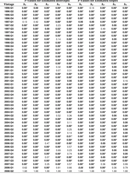
Concerning the parametric model, the p-values of the pooled t-test for the estimated

intercepts and slopes of Vintages K and L, assuming dependence, are presented in Table 2,

and the t-statistics are presented in Table 3. All of the p-values for the estimated intercepts

16 _{The global nonparametric model rejects the null for the two-quarter in-sample forecast horizon for the}

following vintages: V_1997:Q4 to V_1998:Q2 and V_1998:Q4 to V_1999:Q3, and the null is also rejected for the twelve-quarter in-sample forecast horizon for the following vintages: V_1996:Q1 to V_1997:Q1.

are much greater than 0.05 and are closer to unity in a great number of instances, which

means that the null of statistically equivalent estimated intercepts strongly fails to be

rejected. This is also true for the p-values of the pooled t-test for the estimated slope

coefficients of Vintages K and L. Except for h3,the four-quarter in-sample forecast horizon,

for vintages V_2002:Q2 to V_2003:Q4 and for h1, the one-quarter in-sample forecast

horizon, for vintage V_2006:Q4, the null of statistically equivalent estimated slope

coefficients is not rejected. This is not a surprising finding because the differences between

the parametric slopes for Vintage K and L are very close to zero and range between -0.20

and 0.15 as is shown in Graphs 1 and 4.18

So, in regards to the OLS form of the exclusion-from-core inflation persistence

model, the pooled t-test finds for coincidence of the regressions with respect to Vintages K

and L for all five in-sample forecast horizons with a few previously noted exceptions in the

estimated slopes. Thus, the effects of data revisions are essentially lost in this

aggregate-driven regression model.

Concerning the global nonparametric model, Table 4 shows the p-values for the

pooled t-test of the estimated intercepts and estimated slope coefficients, and Table 5

shows the corresponding t-statistics. Comparing Table 4 to Table 2, which is a summary of

the p-values of the parametric model, there are more p-values that are less than 0.05 in the

h1, h2, h3, and h4 in-sample forecast horizons, which range from one-quarter to

eight-quarters. Hence, there are more instances where we reject that the null of coincidence

when using the global nonparametric model as a measure of central tendency especially in

the h1, h2, and h3, in-sample forecast horizons, which ranges from one-quarter to

four-quarters. This indicates that data-revisions are able to be detected, which can be of use for

policy matters in the earlier in-sample forecast horizons even in a model of central

tendency as captured by the global nonparametric regression model.

It should be noted that the Newey-West (1987) standard errors from all the T local

nonparametric regressions are used to form the t-statistic for the global nonparametric

regression model since these residuals are obtained my minimizing the sum of squared

18 _{The shaded areas in Graphs 1 to 6 represent recessions as declared by the NBER and the bold vertical lines}

errors.19 _{When examining Graphs 2 and 5, one can see that the differences between the}

slopes are relatively larger than its parametric counterpart and range between -2.5 and 1.5.

The flexibility of the nonparametric model is able to capture the nonlinearity in

inflation, which is within the current vein of research that finds significant nonlinearity

present in inflation such as Nobay, Paya, and Peel (2007), Chauvet and Tierney (2008),

Choi (2009), and Tierney (2009). In addition, the local conditional nonparametric model is

more efficient than the parametric model, which leads to a better gleaning of information

as it pertains to data revisions as noted by Tierney (2009).

In regards to the effect of data revisions, the strongest effects are captured in the

Tth _{local conditional nonparametric model as is demonstrated in Tables 6 and 7. With a few}

exceptions in each of the in-sample forecast horizons, the p-values of the pooled t-test for

both the estimated intercept and estimated slopes are generally 0.00, which means that the

null of coincidence is strongly rejected with respect to Vintages K and L.20 _{As is shown in}

Graphs 3 and 6, the range in the difference between the Tth _{local conditional estimated}

slopes of Vintage L and Vintage K are larger in magnitude when compared to either the

parametric or global nonparametric model. The range of the observations in Graph 6 is

between -12 and 8, but this is mainly due to the regressions involving the two-quarter

in-sample forecast horizon.21 _{The majority of the differences hover between 1 and -1.}

The fact that data revisions are able to be picked up at the local level has important

policy implications because nonparametrics removes the need to partition a dataset in

order to isolate periods of interest. The Tth _{conditioning observation in the local}

nonparametric regression is automatically incorporated in related periods through the use

of the window width, which functions as a dynamic gain parameter in the weighting

function of Equation (6) by placing a higher weight on observations closer to the

19 _{The global nonparametric regression model is offered as a comparison of central tendency to the}

parametric model, but there is no exact equivalent to the parametric model in the nonparametric methodology.

20 _{For Tables 1 to 6, regardless of the model, the p-value for V_2008:Q2 are all 1.00, and this is due to Vintage} K and Vintage L being one in the same.

21 _{The difference in the estimated slopes for the local conditional nonparametric model is not included for the}

conditioning observation as has been previously stated by Tierney (2009). Thus, as the

results of Tables 6 and 7 have shown, the use of revised data is warranted.

In summary, the flexibility and the efficiency of the local conditional and the global

nonparametric models are able to detect the effects of data revisions, while the parametric

model is unable to do so with just a handful of exceptions.

4.

Conclusion

This paper examines the effects of data revisions in the exclusions-from-core

inflation persistence model in five in-sample forecast horizons in 48 vintages. This

amounts to examining 240 hypothesis tests for coincidence.

Concerning the parametric model, both the estimated intercepts and slopes are not

simultaneously statistically different from zero between Vintage L and Vintage K in any of

the five in-sample forecast horizons. The effects of data revisions are only detected in 16

out of the 240 hypothesis tests of the estimated slope coefficients and in none of the

estimated intercepts. So, in an overwhelming number of regressions, the regressions

produced by OLS are statistically equivalent regardless of vintage. Thus, the effects of data

revisions are essentially lost when using OLS.

With respect to the global nonparametric model, the regressions of the comparison

vintages do not have coincidence as evidenced by having both statistically different

intercepts and slopes in 85 out of the 240 hypothesis tests. This does not include the

results of the comparison where there is only a difference in either the intercept, which

would increase the total by 35, or the slope, which would increase the total by 15.

Concerning the results of the Tth _{local conditional nonparametric model, the comparisons}

find for statistically different intercepts and slopes in 209 out of the 240 regressions.

Thus, data revisions, which are subtle changes in magnitude, can be lost in

aggregation or when outliers dominate such as in the parametric model. With the proper

measuring tool such as the global nonparametric model and especially the Tth _local

conditional nonparametric model, which are flexible and able to provide local time-varying

References

Atkeson CG, Moore AW, and Schaal S. Locally Weighted Learning. Artificial Intelligence Review 1997; 11; 11-73.

Cai Z. Trending Time-Varying Coefficient Time Series Models with Serially Correlated Errors. Journal of Econometrics 2007; 136; 163–188.

Cai Z, Chen R. Flexible Seasonal Time Series Models. In: Fomby BT, Terrell D (Eds), Advances in Econometrics: Honoring Engle and Granger, vol.20(2). Elsevier: Orlando; 2006. p. 63-87.

Cai Z, Fan J, Yao Q. Functional-Coefficient Regression Models for Nonlinear Time Series. Journal of the American Statistical Association 2000; 95(451); 941-956.

Chauvet M, Tierney HLR. Real-Time Changes in Monetary Transmission-A Nonparametric VAR Approach. Working Paper 2008.

Choi CY. Reconsidering the Relationship between Inflation and Relative Price Variability. Working Paper 2009.

Clark TE. Comparing Measures of Core Inflation. Federal Reserve Bank of Kansas City Economic Review 2001; 86(2); 5-31.

Cleveland WS, Devlin JS. Locally Weighted Regression: An Approach to Regression Analysis by Local Fitting.” Journal of the American Statistical Association 1988; 83(403); 596-610.

Cogley T. A Simple Adaptive Measure of Core Inflation. Journal of Money, Credit, and Banking 2002; 43(1); 94-113.

Croushore D. Revisions to PCE Inflation Measures: Implications for Monetary Policy. Federal Reserve Bank of Philadelphia. Working Paper No. 08-8, 2008.

Croushore D, Stark T. A Real-Time Data Set for Macroeconomists. Journal of Econometrics 2001; 105; 111–130.

Croushore D, Stark T. A Real-Time Data Set for Macroeconomists: Does the Data Vintage Matter? The Review of Economics and Statistics 2003; 85(3); 605-617.

Elliott G. Comments on 'Forecasting with a Real-Time Data Set for Macroeconomists'. Journal of Macroeconomics 2002; 24(4); 533-539.

Fan J, Gijbels I. Monographs on Statistics and Applied Probability 66, Local Polynomial Modeling and Its Applications. Chapman and Hall: London; 1996.

Fan J, Yao Q. Efficient Estimation of Conditional Variance Functions in Stochastic Regressions. Biometrika 1998; 85(3); 645-660.

Fujiwara I, Koga M. A Statistical Forecasting Method for Inflation Forecasting: Hitting Every Vector Autoregression and Forecasting under Model Uncertainty. Monetary and Economic Studies, Institute for Monetary and Economic Studies, Bank of Japan 2004; 22(1); 123-142.

Härdle W, Linton O. Applied Nonparametric Methods. In: Engle RF, Mc Fadden DL (Eds), Handbook of Econometrics, vol.IV. North-Holland: Amsterdam; 1994.

Härdle W, Lütkepohl H, Chen R. A Review of Nonparametric Time Series Analysis. International Statistical Review/Revue Internationale de Statistique 1997; 65(1); 49-72.

Härdle W, Tsybakov, A. Local Polynomial Estimator of the Volatility Function in Nonparametric Autoregression. Journal of Econometrics 1997; 81; 223-242.

Howell DC. Fundamental Statistics for the Behavioral Sciences (6th International Edition). Thompson Learning: London; 2007.

Johnson M. Core Inflation: A Measure of Inflation for Policy Purposes. Proceedings from Measures of Underlying Inflation and their Role in Conduct of Monetary Policy-Workshop of Central Model Builders at Bank for International Settlements, February 1999.

Kleinbaum DG, Kupper LL. Applied Regression Analysis and Other Multivariable Methods. Duxbury Press: Belmont; 1978.

Lafléche T, Armour, J. Evaluating Measures of Core Inflation. Bank of Canada Review, Summer 2006.

Lanne M. Nonlinear Dynamics of Interest Rate and Inflation. Journal of Applied Econometrics 2006; 21(8); 1157-1168.

Marron JS. Automatic Smoothing Parameter Selection: A Survey. Empirical Economics 1988; 13; 187-208.

Nobay B, Paya I, Peel DA. Inflation Dynamics in the US -A Nonlinear Perspective. Working Paper, 2007.

Pagan A, Ullah A. Nonparametric Econometrics. Cambridge University Press: Cambridge; 1999.

Rich R, Steindel C. A Review of Core Inflation and an Evaluation of Its Measures. Federal Reserve Bank of New York Staff Report No. 236, December 2005.

Robinson PM. Inference Without-Smoothing in the Presence of Autocorrelation. Econometrica 1998; 66(5); 1163-1182.

Ruppert D, Wand MP. Multivariate Locally Weighted Least Squares Regression. The Annals of Statistics 1994; 22; 1346-1370.

Tierney HLR. A Nonparametric Study of Inflation Persistence with Real-Time Data: Using Exclusions-from-Core Measures of Inflation. VDM Verlag: Saarbrücken; 2009.

Wand MP, Jones MC. Kernel Smoothing. Chapman & Hall: London; 1995.

-.1 .0 .1 .2 .3 .4 .5 .6 .7 .8

96 97 98 99 00 01 02 03 04 05 06 07 08

Slope Vintage K Slope V_2008:Q2 Difference b/w Slopes Graph 1: Parametric Model In-Sample Forecast Horizon--1 Quarter

-0.5 0.0 0.5 1.0 1.5 2.0

96 97 98 99 00 01 02 03 04 05 06 07 08

Slope Vintage K Slope V_2008:Q2 Difference b/w Slopes

-6 -4 -2 0 2 4 6

1996 1997 1998 1999 2000 2001 2002 2003 2004 2005 2006 2007 2008

Slope Vintage K Slope V_2008:Q2 Difference b/w Slopes

Graph 3: Local Conditional Nonparametric Model In-Sample Forecast Horizon--1 Quarter

(Conditional on Last Obs of Vintage K)

-.25 -.20 -.15 -.10 -.05 .00 .05 .10 .15

96 97 98 99 00 01 02 03 04 05 06 07 08

h1-(1 Quarter) h2-(2 Quarters) h3-(4 Quarters) h4-(8 Quarters) h5-(12 Quarters) Graph 4: Parametric Model

-2.5 -2.0 -1.5 -1.0 -0.5 0.0 0.5 1.0 1.5

96 97 98 99 00 01 02 03 04 05 06 07 08

h1-(1 Quarter) h2-(2 Quarters) h3-(4 Quarters) h4-(8 Quarters) h5-(12 Quarters)

Graph 5: Global (Averaged) Nonparametric Model Difference in Slopes

(V_2008:Q2 - Vintage K)

-12 -8 -4 0 4 8

96 97 98 99 00 01 02 03 04 05 06 07 08

h1-(1 Quarter) h2-(2 Quarters) h3-(4 Quarters) h4-(8 Quarters) h5-(12 Quarters)

Graph 6: Local Conditional Nonparametric Model (Conditional on Last Obs of Vintage K)

Table 1

Sample Size and In-Sample Forecast Horizons

Horizon # of Obs. Sample Period Vintages

Full Sample 48 to 98 1983:Q4-2008:Q1 1996:Q1- 2008:Q2

h1 (1 quarter) 47 to 96 1984:Q1-2007:Q4 1996:Q1- 2007:Q4

h2 (2 quarters) 46 to 95 1984:Q1-2007:Q3 1996:Q1- 2007:Q3

h3 (4 quarters) 44 to 93 1984:Q1-2007:Q1 1996:Q1- 2007:Q1

h4 (8 quarters) 40 to 89 1984:Q1-2004:Q1 1996:Q1- 2006:Q1

Table 2

P-Values for the Hypothesis Test for Coincidence—Parametric Model

P-Values for Estimated Intercepts P-Values for Estimated Slopes Vintage h1 h2 h3 h4 h5 h1 h2 h3 h4 h5

1996:Q1 0.88 0.86 0.84 0.85 0.95 0.72 0.16 0.33 0.94 0.92

1996:Q2 0.82 0.94 0.63 0.76 0.90 0.89 0.17 0.27 0.99 0.93

1996:Q3 0.95 0.73 0.64 0.80 0.93 0.83 0.10 0.22 0.98 0.91

1996:Q4 0.92 0.69 0.61 0.82 0.92 0.92 0.10 0.18 0.95 0.91

1997:Q1 0.89 0.86 0.62 0.83 0.90 0.97 0.15 0.18 0.92 0.93

1997:Q2 0.89 0.97 0.70 0.74 0.84 0.98 0.35 0.23 0.88 0.82

1997:Q3 0.99 0.68 0.96 0.90 1.00 0.78 0.13 0.38 0.99 0.97

1997:Q4 0.96 0.72 0.87 0.91 0.97 0.80 0.15 0.34 1.00 0.95

1998:Q1 0.99 0.76 0.82 0.92 1.00 0.83 0.16 0.27 0.99 0.96

1998:Q2 0.98 0.87 0.73 0.89 0.95 0.84 0.19 0.24 0.99 0.91

1998:Q3 0.93 0.83 0.76 0.76 0.85 0.86 0.27 0.48 0.97 0.89

1998:Q4 0.98 0.86 0.64 0.73 0.83 0.81 0.30 0.44 0.96 0.89

1999:Q1 0.99 0.93 0.63 0.72 0.82 0.81 0.30 0.42 0.96 0.88

1999:Q2 0.96 0.89 0.60 0.62 0.82 0.82 0.31 0.28 0.90 0.84

1999:Q3 0.95 0.80 0.66 0.60 0.83 0.77 0.29 0.36 0.97 0.87

2000:Q2 0.75 0.99 0.49 0.79 0.85 0.49 0.74 0.00 0.86 0.51

2000:Q3 0.88 0.97 0.55 0.85 0.92 0.59 0.84 0.00 0.89 0.52

2000:Q4 0.87 0.90 0.60 0.83 0.92 0.56 0.70 0.00 0.88 0.59

2001:Q1 0.86 0.95 0.60 0.83 0.92 0.54 0.82 0.00 0.88 0.59

2001:Q2 0.82 0.90 0.68 0.80 0.93 0.52 0.93 0.00 0.93 0.58

2001:Q3 0.70 0.60 0.62 0.88 0.90 0.52 0.97 0.00 0.86 0.61

2001:Q4 0.69 0.19 0.31 0.75 0.83 0.46 0.25 0.00 0.70 0.62

2002:Q1 0.86 0.45 0.33 0.79 0.86 0.39 0.27 0.00 0.74 0.61

2002:Q2 0.81 0.83 0.39 0.73 0.83 0.52 0.54 0.00 0.64 0.60

2002:Q3 0.80 0.84 0.68 0.80 0.88 0.51 0.52 0.00 0.77 0.56

2002:Q4 0.85 0.93 0.78 0.80 0.89 0.52 0.86 0.00 0.76 0.60

2003:Q1 0.88 0.97 0.73 0.78 0.91 0.51 0.75 0.00 0.75 0.64

2003:Q2 0.78 0.90 0.71 0.76 0.92 0.45 0.75 0.00 0.73 0.68

2003:Q3 0.90 0.86 0.73 0.82 0.89 0.61 0.80 0.00 0.80 0.62

2003:Q4 0.90 0.95 0.73 0.86 0.88 0.64 0.41 0.00 0.73 0.64

2004:Q1 0.86 0.57 0.73 0.93 0.92 0.89 0.49 0.68 0.84 0.91

2004:Q2 1.00 0.88 0.81 0.94 0.92 0.77 0.78 0.76 0.92 0.91

2004:Q3 0.89 0.86 0.83 0.92 0.94 0.73 0.62 0.91 0.96 0.90

2004:Q4 0.83 0.72 0.81 0.87 0.91 0.88 0.45 0.93 0.98 0.95

2005:Q1 0.97 0.82 0.81 0.87 0.90 0.64 0.60 0.95 0.99 0.97

2005:Q2 0.84 0.99 0.85 0.86 0.90 0.56 0.80 0.99 0.95 0.99

2005:Q3 0.97 0.98 1.00 0.99 0.98 0.78 0.61 0.85 0.93 0.97

2005:Q4 0.81 0.91 0.97 0.97 0.96 0.66 0.73 0.96 0.97 0.97

2006:Q1 1.00 0.94 0.94 0.98 0.96 0.98 0.81 0.99 0.96 0.96

2006:Q2 0.83 0.91 0.99 0.98 0.97 0.74 0.71 0.99 0.97 0.99

2006:Q3 0.97 0.98 0.99 1.00 1.00 0.09 0.69 0.99 1.00 0.97

2006:Q4 0.96 0.98 1.00 0.99 0.99 0.03 0.65 0.97 0.99 0.97

2007:Q1 0.97 1.00 0.99 0.99 0.99 0.66 0.73 0.96 0.99 0.98

2007:Q2 1.00 0.99 0.97 0.99 0.98 0.79 0.77 1.00 0.98 0.99

2007:Q3 0.99 1.00 1.00 1.00 1.00 0.99 0.99 0.99 1.00 1.00

2007:Q4 0.98 0.99 0.99 0.99 1.00 0.94 0.99 1.00 0.98 1.00

2008:Q1 0.99 1.00 1.00 1.00 1.00 1.00 0.99 0.99 1.00 1.00

Table 3

T-Statistics for the Hypothesis Test for Coincidence—Parametric Model

T-Statistics for Estimated Intercepts T-Statistics for Estimated Slopes Vintage h1 h2 h3 h4 h5 h1 h2 h3 h4 h5

1996:Q1 0.15 0.18 0.20 0.19 0.06 0.36 1.42 0.98 0.07 0.11

1996:Q2 0.23 0.08 0.48 0.30 0.13 0.14 1.39 1.12 0.01 0.09

1996:Q3 0.06 0.34 0.48 0.26 0.09 0.21 1.66 1.25 0.03 0.11

1996:Q4 0.10 0.41 0.52 0.23 0.10 0.10 1.69 1.35 0.06 0.12

1997:Q1 0.14 0.18 0.49 0.22 0.12 0.04 1.47 1.37 0.10 0.09

1997:Q2 0.14 0.04 0.38 0.33 0.21 0.02 0.94 1.23 0.15 0.23

1997:Q3 0.02 0.42 0.06 0.13 0.00 0.28 1.56 0.89 0.01 0.04

1997:Q4 0.05 0.35 0.16 0.12 0.04 0.26 1.44 0.97 0.01 0.07

1998:Q1 0.02 0.31 0.23 0.10 0.01 0.22 1.42 1.11 0.01 0.05

1998:Q2 0.02 0.16 0.35 0.14 0.06 0.20 1.31 1.19 0.01 0.12

1998:Q3 0.08 0.21 0.31 0.31 0.19 0.18 1.12 0.71 0.04 0.14

1998:Q4 0.02 0.18 0.47 0.34 0.22 0.24 1.06 0.78 0.05 0.14

1999:Q1 0.01 0.09 0.49 0.36 0.23 0.24 1.06 0.81 0.05 0.15

1999:Q2 0.05 0.14 0.53 0.50 0.22 0.23 1.03 1.09 0.12 0.20

1999:Q3 0.06 0.26 0.44 0.53 0.21 0.29 1.08 0.92 0.04 0.17

2000:Q2 0.32 0.01 0.70 0.27 0.19 0.69 0.33 3.39 0.18 0.66

2000:Q3 0.15 0.03 0.61 0.19 0.11 0.55 0.21 4.93 0.14 0.65

2000:Q4 0.16 0.13 0.53 0.22 0.10 0.59 0.38 6.44 0.15 0.54

2001:Q1 0.17 0.06 0.52 0.22 0.10 0.62 0.23 10.91 0.15 0.54

2001:Q2 0.23 0.13 0.41 0.25 0.09 0.64 0.09 6.61 0.09 0.55

2001:Q3 0.39 0.52 0.50 0.15 0.13 0.65 0.04 3.03 0.18 0.51

2001:Q4 0.40 1.31 1.01 0.32 0.22 0.75 1.16 4.57 0.40 0.49

2002:Q1 0.17 0.76 0.98 0.27 0.18 0.86 1.10 5.58 0.34 0.51

2002:Q2 0.24 0.22 0.86 0.35 0.22 0.65 0.61 4.39 0.47 0.54

2002:Q3 0.26 0.20 0.42 0.26 0.16 0.66 0.65 3.42 0.29 0.59

2002:Q4 0.19 0.09 0.28 0.25 0.13 0.64 0.17 3.48 0.30 0.52

2003:Q1 0.15 0.03 0.34 0.28 0.11 0.65 0.32 5.29 0.32 0.47

2003:Q2 0.28 0.12 0.37 0.31 0.11 0.76 0.32 3.26 0.34 0.42

2003:Q3 0.13 0.17 0.34 0.22 0.14 0.51 0.26 3.16 0.26 0.49

2003:Q4 0.12 0.06 0.35 0.18 0.15 0.46 0.83 3.42 0.34 0.47

2004:Q1 0.18 0.57 0.35 0.09 0.10 0.14 0.69 0.41 0.20 0.12

2004:Q2 0.00 0.15 0.25 0.07 0.10 0.30 0.28 0.31 0.11 0.12

2004:Q3 0.14 0.18 0.21 0.10 0.08 0.35 0.49 0.11 0.05 0.12

2004:Q4 0.21 0.35 0.24 0.17 0.12 0.15 0.76 0.09 0.02 0.07

2005:Q1 0.03 0.23 0.24 0.17 0.13 0.46 0.52 0.07 0.01 0.04

2005:Q2 0.20 0.01 0.19 0.18 0.12 0.59 0.25 0.01 0.07 0.01

2005:Q3 0.04 0.03 0.00 0.01 0.03 0.28 0.52 0.19 0.09 0.03

2005:Q4 0.24 0.11 0.04 0.03 0.05 0.44 0.35 0.06 0.04 0.04

2006:Q1 0.00 0.08 0.07 0.03 0.05 0.02 0.25 0.01 0.05 0.05

2006:Q2 0.22 0.11 0.02 0.02 0.03 0.33 0.38 0.01 0.04 0.02

2006:Q3 0.04 0.03 0.02 0.00 0.01 1.74 0.40 0.02 0.01 0.04

2006:Q4 0.05 0.03 0.01 0.01 0.01 2.29 0.46 0.04 0.01 0.04

2007:Q1 0.04 0.00 0.01 0.02 0.01 0.44 0.34 0.05 0.02 0.03

2007:Q2 0.00 0.02 0.04 0.02 0.02 0.27 0.29 0.00 0.03 0.02

2007:Q3 0.01 0.01 0.00 0.00 0.00 0.01 0.02 0.01 0.01 0.01

2007:Q4 0.03 0.02 0.01 0.01 0.00 0.07 0.02 0.01 0.03 0.00

2008:Q1 0.01 0.00 0.00 0.00 0.00 0.00 0.01 0.01 0.00 0.00

Table 4

P-Values for the Hypothesis Test for Coincidence—Global Nonparametric Model

P-Values for Estimated Intercepts P-Values for Estimated Slopes Vintage h1 h2 h3 h4 h5 h1 h2 h3 h4 h5

1996:Q1 0.31 0.15 0.00 0.06 0.06 0.00 0.52 0.89 0.00 0.17

1996:Q2 0.37 0.18 0.00 0.10 0.07 0.00 0.17 0.70 0.00 0.11

1996:Q3 0.65 0.97 0.00 0.08 0.05 0.10 0.00 0.40 0.00 0.79

1996:Q4 0.03 0.21 0.00 0.05 0.06 0.65 0.00 0.96 0.00 0.06

1997:Q1 0.02 0.00* 0.00 0.05 0.05 0.99 0.00* 0.05 0.00 0.00

1997:Q2 0.00 0.66 0.00* 0.75 0.22 0.55 0.00 0.00* 0.32 0.06

1997:Q3 0.00 0.00* 0.00* 0.74 0.49 0.86 0.00* 0.00* 0.02 0.89

1997:Q4 0.00 0.00* 0.00* 0.75 0.35 0.54 0.00* 0.00* 0.05 0.03

1998:Q1 0.00 0.00* 0.00* 0.74 0.27 0.62 0.00* 0.00* 0.11 0.13

1998:Q2 0.00 0.00* 0.00* 0.64 0.22 0.65 0.00* 0.00* 0.28 0.51

1998:Q3 0.00 0.22 0.00* 0.12 0.16 0.38 0.00 0.00* 0.68 0.87

1998:Q4 0.00 0.00* 0.00* 0.40 0.13 0.20 0.00* 0.00* 0.71 0.82

1999:Q1 0.00 0.00* 0.00* 0.34 0.11 0.34 0.00* 0.00* 0.50 0.78

1999:Q2 0.00 0.00* 0.00* 0.50 0.09 0.43 0.00* 0.00* 0.29 0.94

1999:Q3 0.00 0.00* 0.00* 0.22 0.07 0.98 0.00* 0.00* 0.64 0.90

2000:Q2 0.02 0.00* 0.00* 0.08 0.00 0.61 0.00* 0.00* 0.60 0.14

2000:Q3 0.07 0.00* 0.00* 0.10 0.01 0.90 0.00* 0.00* 0.66 0.63

2000:Q4 0.05 0.00* 0.00* 0.10 0.02 0.98 0.00* 0.00* 0.63 0.54

2001:Q1 0.14 0.00* 0.00* 0.09 0.02 0.68 0.00* 0.00* 0.65 0.53

2001:Q2 0.17 0.00* 0.00* 0.17 0.10 0.99 0.00* 0.00* 0.59 0.06

2001:Q3 0.09 0.00* 0.00* 0.41 0.07 0.78 0.00* 0.02* 0.70 0.15

2001:Q4 0.06 0.00* 0.00 0.32 0.04 0.98 0.00* 0.10 0.75 0.25

2002:Q1 0.04 0.00* 0.00* 0.28 0.03 0.77 0.00* 0.01* 0.89 0.15

2002:Q2 0.00 0.00* 0.00* 0.45 0.02 0.32 0.00* 0.03* 0.92 0.13

2002:Q3 0.00* 0.00* 0.00* 0.50 0.02 0.00* 0.00* 0.02* 0.75 0.06

2002:Q4 0.00* 0.00* 0.00* 0.62 0.03 0.00* 0.00* 0.04* 0.51 0.12

2003:Q1 0.00* 0.00* 0.00* 0.61 0.03 0.00* 0.00* 0.00* 0.56 0.15

2003:Q2 0.00* 0.00* 0.00* 0.60 0.05 0.00* 0.00* 0.00* 0.69 0.26

2003:Q3 0.00* 0.00* 0.00* 0.46 0.06 0.00* 0.00* 0.00* 0.63 0.68

2003:Q4 0.00* 0.00* 0.00* 0.39 0.05 0.00* 0.00* 0.00* 0.67 0.49

2004:Q1 0.00* 0.00* 0.01 0.42 0.93 0.00* 0.00* 0.07 0.20 0.69

2004:Q2 0.00* 0.00* 0.00* 0.46 0.95 0.00* 0.00* 0.00* 0.23 0.68

2004:Q3 0.00* 0.00* 0.00* 0.90 0.89 0.00* 0.00* 0.00* 0.76 0.85

2004:Q4 0.02 0.00* 0.00* 0.77 0.88 0.06 0.00* 0.00* 0.97 0.96

2005:Q1 0.03 0.00* 0.00* 0.77 0.88 0.33 0.00* 0.00* 0.92 0.87

2005:Q2 0.00 0.00* 0.00* 0.00* 0.86 0.05 0.00* 0.00* 0.00* 0.95

2005:Q3 0.00* 0.00* 0.00* 0.65 0.94 0.00* 0.00* 0.00* 0.91 0.90

2005:Q4 0.00* 0.00* 0.00* 0.78 0.90 0.00* 0.00* 0.00* 0.58 0.97

2006:Q1 0.00* 0.00* 0.00* 0.79 0.89 0.00* 0.00* 0.00* 0.60 0.97

2006:Q2 0.00* 0.00* 0.00* 0.83 0.46 0.00* 0.00* 0.00* 0.64 0.25

2006:Q3 0.00* 0.81 0.50 0.84 0.49 0.00* 0.72 0.70 0.62 0.26

2006:Q4 0.00* 0.78 0.97 0.83 0.48 0.00* 0.70 0.87 0.61 0.26

2007:Q1 0.01* 0.90 0.95 0.72 0.48 0.00* 1.00 0.97 0.36 0.29

2007:Q2 0.00* 0.94 0.95 0.74 0.36 0.00* 0.97 0.54 0.43 0.10

2007:Q3 0.96 0.91 0.97 0.98 0.99 0.97 0.96 0.96 0.96 0.96

2007:Q4 0.54 0.93 0.98 0.98 0.99 0.68 0.96 0.98 0.98 0.99

2008:Q1 0.99 0.93 0.96 1.00 0.99 0.97 0.96 0.98 1.00 0.99

Table 5

T-Statistics for the Hypothesis Test for Coincidence—Global Nonparametric Model

T-Statistics for Estimated Intercepts T-Statistics for Estimated Slopes Vintage h1 h2 h3 h4 h5 h1 h2 h3 h4 h5

1996:Q1 1.03 1.47 9.80 1.91 2.01 4.95 0.65 0.14 4.57 1.42

1996:Q2 0.90 1.37 10.82 1.68 1.91 4.74 1.39 0.39 5.02 1.67

1996:Q3 0.46 0.04 11.37 1.81 2.12 1.70 4.75 0.86 5.00 0.27

1996:Q4 2.24 1.28 12.16 2.02 1.97 0.46 6.07 0.05 4.55 2.02

1997:Q1 2.42 4.05* 11.32 2.00 2.11 0.01 8.91* 1.98 5.37 4.01

1997:Q2 10.60 0.44 9.63* 0.32 1.25 0.60 4.77 3.47* 1.02 1.92

1997:Q3 7.90 127.58* 8.21* 0.33 0.70 0.18 11.04* 5.24* 2.57 0.14

1997:Q4 7.09 106.32* 9.11* 0.32 0.95 0.62 9.59* 4.26* 2.03 2.21

1998:Q1 6.68 94.35* 10.14* 0.34 1.11 0.50 9.00* 5.38* 1.64 1.53

1998:Q2 6.59 86.44* 10.42* 0.47 1.25 0.45 9.44* 4.64* 1.10 0.66

1998:Q3 7.95 1.23 8.75* 1.60 1.41 0.89 3.14 3.38* 0.42 0.17

1998:Q4 5.88 82.64* 10.87* 0.85 1.56 1.31 10.74* 3.44* 0.37 0.23

1999:Q1 5.95 77.00* 11.61* 0.97 1.61 0.96 11.15* 3.21* 0.68 0.28

1999:Q2 6.09 72.06* 12.35* 0.68 1.71 0.79 12.44* 5.26* 1.07 0.07

1999:Q3 6.32 77.08* 9.84* 1.24 1.85 0.03 9.38* 4.80* 0.47 0.12

2000:Q2 2.43 14.09* 11.48* 1.80 3.37 0.51 8.98* 3.10* 0.53 1.50

2000:Q3 1.87 12.53* 14.00* 1.68 2.63 0.13 7.71* 13.49* 0.45 0.49

2000:Q4 1.96 11.63* 13.90* 1.69 2.48 0.03 8.28* 18.51* 0.49 0.61

2001:Q1 1.48 11.29* 15.17* 1.72 2.46 0.41 7.95* 14.10* 0.46 0.64

2001:Q2 1.40 18.74* 12.86* 1.40 1.71 0.02 11.60* 4.05* 0.55 1.94

2001:Q3 1.70 19.09* 11.13* 0.83 1.90 0.28 11.52* 2.31* 0.39 1.47

2001:Q4 1.92 53.18* 12.51 1.02 2.20 0.03 14.75* 1.69 0.32 1.17

2002:Q1 2.05 39.96* 13.62* 1.10 2.21 0.29 14.50* 2.79* 0.14 1.46

2002:Q2 13.23 24.71* 11.65* 0.76 2.36 1.00 11.47* 2.24* 0.10 1.56

2002:Q3 11.12* 89.07* 11.39* 0.68 2.43 3.96* 37.87* 2.48* 0.33 1.94

2002:Q4 11.49* 72.44* 11.13* 0.50 2.33 3.50* 36.74* 2.06* 0.67 1.59

2003:Q1 11.61* 56.29* 28.87* 0.52 2.30 3.94* 35.82* 11.31* 0.59 1.46

2003:Q2 11.81* 66.80* 24.51* 0.54 2.04 3.30* 37.91* 10.40* 0.41 1.14

2003:Q3 4.28* 54.07* 24.48* 0.75 1.98 7.34* 33.82* 8.44* 0.48 0.42

2003:Q4 4.03* 6.10* 24.90* 0.88 2.04 6.84* 20.29* 9.17* 0.43 0.70

2004:Q1 16.18* 29.47* 2.80 0.81 0.08 4.11* 17.37* 1.84 1.31 0.41

2004:Q2 20.81* 20.34* 8.39* 0.74 0.06 6.15* 12.41* 6.14* 1.22 0.42

2004:Q3 4.45* 25.14* 16.33* 0.13 0.14 5.14 18.74* 15.21* 0.31 0.18

2004:Q4 2.38 27.39* 17.31* 0.29 0.15 1.91 21.37* 16.65* 0.03 0.04

2005:Q1 2.24 26.64* 16.55* 0.30 0.15 0.98 20.52* 16.47* 0.10 0.16

2005:Q2 3.43 27.06* 16.63* 12.16* 0.18 2.00 20.06* 16.44* 11.46* 0.06

2005:Q3 12.44* 18.88* 5.44* 0.45 0.07 10.01* 11.52* 5.99* 0.12 0.12

2005:Q4 58.68* 17.11* 4.58* 0.28 0.12 39.88* 10.22* 3.80* 0.56 0.04

2006:Q1 33.87* 20.65* 4.36* 0.27 0.13 25.26* 13.50* 3.45* 0.52 0.04

2006:Q2 28.78* 19.66* 4.64* 0.22 0.75 20.59* 14.05* 3.75* 0.47 1.16

2006:Q3 13.13* 0.24 0.67 0.21 0.69 26.81* 0.37 0.38 0.50 1.14

2006:Q4 20.65* 0.28 0.04 0.21 0.71 31.55* 0.39 0.16 0.51 1.14

2007:Q1 2.77* 0.13 0.06 0.36 0.71 3.42* 0.00 0.04 0.93 1.06

2007:Q2 12.75* 0.07 0.06 0.34 0.93 22.38* 0.04 0.62 0.80 1.67

2007:Q3 0.05 0.12 0.04 0.02 0.02 0.03 0.05 0.06 0.05 0.05

2007:Q4 0.62 0.08 0.03 0.02 0.01 0.41 0.05 0.02 0.02 0.01

2008:Q1 0.01 0.09 0.06 0.00 0.01 0.04 0.05 0.03 0.00 0.01