Munich Personal RePEc Archive
Estimating Monetary Policy Reaction
Functions Using Quantile Regressions
Wolters, Maik Hendrik
Goethe University Frankfurt
13 July 2010
Online at
https://mpra.ub.uni-muenchen.de/23857/
Estimating Monetary Policy Reaction Functions Using Quantile
Regressions
Maik H. Wolters∗ Goethe University Frankfurt
July 2010
Abstract
Monetary policy rule parameters are usually estimated at the mean of the interest rate distribution conditional on inflation and an output gap. This is an incomplete description of monetary policy reactions when the parameters are not uniform over the conditional distribution of the interest rate. I use quantile regressions to estimate parameters over the whole conditional distribution of the Federal Funds Rate. Inverse quantile regressions are applied to deal with endogeneity. Real-time data of inflation forecasts and the output gap are used. I find significant and systematic variations of parameters over the conditional distribution of the interest rate.
Keywords: monetary policy rules, IV quantile regression, real-time data JEL-Codes: C14, E52, E58
∗I am grateful for helpful comments by Tim Oliver Berg, Tobias Cwik, Stefan Gerlach, Sebastian Schmidt and Volker
1
Introduction
Policy rules of the form proposed by Taylor (1993) to understand the interest rate setting of the Federal Open Market Committee (FOMC) in the late 1980s and early 1990s have been used as a tool to study historical monetary policy decisions. Although estimated versions describe monetary policy in the U.S. quite well, in reality the Federal Reserve does not follow a policy rule mechanically: ”The monetary policy of the Federal Reserve has involved varying degrees of rule- and discretionary-based modes of operation over time,” (Greenspan, 1997). This raises the question how the FOMC responds to inflation and the output gap during periods that cannot be described accurately by a policy rule. Except anecdotal descriptions of some episodes (e.g. Taylor, 1993; Poole, 2006) there appears to be a lack of studies that analyze deviations from Taylor’s rule systematically and quantitatively.
In addition to changes between discretionary and rule-based policy regimes, economic theory provides several reasons for deviating at least at times from a linear policy rule framework. First, asymmetric central bank preferences can lead in an otherwise linear model to a nonlinear policy reaction function (Gerlach, 2000; Surico, 2007; Cukierman and Muscatelli, 2008). A nonlinear policy rule can be optimal when the central bank has a quadratic loss function, but the economy is nonlinear (Schaling, 1999; Dolado, Maria-Dolores, and Naveira, 2005). Even in a linear economy with symmetric central bank preferences an asymmetric policy rule can be optimal if there is uncer-tainty about specific model parameters: Meyer, Swanson, and Wieland (2001) analyse unceruncer-tainty regarding the NAIRU and Tillmann (2010) studies optimal policy with uncertainty about the slope of the Phillips Curve. Finally, when interest rates approach the zero lower bound, responses to inflation might increase to avoid the possibility of deflation (Orphanides and Wieland, 2000; Kato and Nishiyama, 2005; Tomohiro Sugo, 2005; Adam and Billi, 2006). Despite these concerns in the empirical literature estimation of linear policy rules prevails with only few exceptions.
the period 1969 through 2002 confirming the breakpoint test results of Orphanides (2004).
The results indicate that policy parameters fluctuate significantly over the conditional distribution of the Federal Funds Rate. These deviations from the parameter estimates at the conditional mean of the interest rate are systematic: inflation reactions and the interest rate smoothing parameter increase and output gap responses decrease over the conditional distribution of the interest rate. The results are robust to variations in the sample. They indicate that the FOMC has sought to stabilize inflation more and output less when setting the interest rate higher than implied by the estimated policy rule and vice versa. Thus, a fraction of deviations from an estimated linear policy rule are possibly not caused by policy shocks, but by systematic changes in the policy parameters or an asymmetric policy rule.
Having analyzed how the Federal Reserve sets interest rates when deviating from the conditional mean it is of interest whether these deviations are related to the business cycle. I estimate for each observation at which quantile of its conditional distribution the interest rate is located. Knowing the parameters at the mean and at the estimated quantile for each observation of the sample one can decompose overall deviations of the Federal Funds Rate from a linear policy rule into differences in the inflation reaction, the output gap reaction, the reaction to the lagged interest rate and differences in the constant. I find anticyclical deviations of monetary policy from a linear policy rule with respect to the output gap response for the Volcker-Greenspan era. Together with a decreasing output gap parameter over the conditional distribution of the interest rate one can conclude that the Fed reacted more to the output gap during recessions than during expansions. This leads to lower interest rates than implied by a linear policy rule during recessions. A recession avoidance preference of the FOMC found by Cukierman and Muscatelli (2008) is thus confirmed.
The remainder of this paper is organized as follows: Section 2 presents the real-time dataset. Section 3 presents estimation results for standard methods. Afterwards, section 4 gives an overview on quantile regression methods. In section 5 the quantile regression results are presented and discussed. Section 6 links parameter variations to the business cycle. Finally, section 7 concludes.
2
Data
I use real-time data from 1969 through 2003 that were available at the Federal Reserve at the time of policy decisions.1 For expected inflation I compute year-on-year inflation forecasts four quarters ahead of the policy decisions using four successive quarter-on-quarter forecasts of the GDP/GNP
flator computed by Federal Reserve staff for the Greenbook.2 Data sources for output gap nowcasts as used by the Federal Reserve are described by Orphanides (2004) in detail. From 1969 until 1976 output gap estimates were computed by the Council of Economic Advisors. Afterwards the Federal Reserve staff started to compute an own output gap series. The output gap estimates by the Fed were not officially published in the Greenbook, but were used to prepare projections of other variables included in the Greenbook. Finally, the interest rate is measured as the annual effective yield of the Federal Funds Rate.
An important aspect of the analysis is that the different data series correspond exactly to the infor-mation available at the dates of the specific FOMC meetings. I use observations of as many FOMC meetings as possible to describe U.S. monetary policy with high accurracy. Therefore, the frequency of the observations is not equally spaced and varies over the sample: data from 1969 to 1971 is an-nual, the observations for 1972 and 1973 are seminanan-nual, data until 1987 is quarterly and for most years of the remaining sample there is data available for eight FOMC meetings per year. In addition, I create quarterly spaced data for robustness checks. A plot of the data is shown in figure 1. It is no-ticeable that the Fed perceived the output gap to be negative in real-time for large parts of the sample.
1970 1975 1980 1985 1990 1995 2000
−15 −10 −5 0 5 10 15
Federal Funds Rate
Inflation Forecast
[image:5.612.85.528.347.465.2]Output Gap
Figure 1:Federal Funds Rate, Inflation Forecasts and Output Gap Nowcasts. Notes: Inflation forecasts reflect percentage year-over-year changes in the GDP/GNP deflator. Output gap nowcasts measure deviations of real output from potential output in percent. The interest rate is the annual effective yield of Federal Funds Rate.
3
Least Squares Regressions
I estimate a monetary policy rule of the form:
it =ρit−1+ (1−ρ)(i∗+β(πt+4|t−π∗) +γyt) +εt, (1) 2To be sure, these forecasts need not to coinicide with the forecasts of the FOMC members. Orphanides and Wieland
whereit is the nominal short term interest rate,i∗is the targeted nominal rate,πt+4|t is a
four-quarter-ahead inflation forecast, π∗ is the inflation target, y
t is the output gap andεt is a policy shock. ρ,
β andγ are policy parameters. Thus, the Federal Funds Rate responds systematically to deviations of the inflation forecast from a target and to the output gap. The interest rate is adjusted gradually to its target. Orphanides (2001) shows that forward-looking policy rules provide a better description of U.S. monetary policy than backward-looking rules in the sense that they do not violate the Taylor principle when being estimated with real-time data.
The nominal interest rate target can be decomposed into the targeted real interest rate and the inflation target:i∗=r∗+π∗. To use linear estimation techniques equation (1) is rewritten:
it =α0+αiit−1+αππt+4|t+αyyt+εt, (2)
whereα0= (1−ρ)(r∗+ (1−β)π∗), αi =ρ, απ = (1−ρ)β andαy = (1−ρ)γ. Parameters can
be estimated at the conditional expected value of the Federal Funds Rate with standard methods like ordinary least squares (OLS) or two-stage least squares (TSLS) to handle endogeneity problems:
E(it|it−1,πt+4|t,yt) =α0+αiit−1+αππt+4|t+αyyt. (3)
3.1 Specification Tests
Table 1:p-Values of Subsample Stability Tests
OLS TSLS
Parameters all data quarterly data all data quarterly data
All 0.12 0.14 0.05 0.06
α0 0.17 0.15 0.09 0.09
απ 0.09 0.08 0.03 0.03
αy 0.02 0.01 0.01 0.01
αi 0.10 0.11 0.20 0.19
α0(αyvaries) 0.67 0.72 0.91 0.78
απ(αyvaries) 0.95 0.94 0.38 0.43
αi(αyvaries) 0.81 0.90 0.34 0.49
Notes: The entries show p-values of parameter stability tests across the subsamples 1969:4-1979:2 and 1979:3-2003:4. Test results are shown for all available FOMC meetings and for quarterly data. Row 1 examines the null hypothesis of joint constancy of all parameters. Rows 2-5 test the null hypothesis that the specific parameter shown is constant, under the assumption that remaining parameters are constant. Rows 6-8 test the null hypothesis that the specific parameter shown is constant whenαyis allowed to vary and remaining parameters are constant.
Table 1 shows that the null hypothesis of no structural break cannot be rejected. However, as the p-values in the case of the TSLS estimates are close to rejection I investigate if there is a structural break in specific parameters. The hypothesis of no structural breaks in the constant and the interest rate smoothing parameters are accepted, while the evidence is mixed for the inflation parameter. Constancy of the output gap response parameter is rejected in all cases. Allowing this parameter to vary, the null hypothesis of no structural break in all the other parameters is accepted. Based on this, I estimate policy rules over the period 1969:4-2003:4, allowing for a structural change ofαyin 1979:3.
[image:7.612.83.524.561.657.2]Policy rule estimates using revised data of inflation and the output gap have relied on instrumental variable methods, (see, e.g., Clarida, Gal´ı, and Gertler, 1998). In contrast, the literature using real-time data has not used instrumental variable methods as inflation forecasts and output gap nowcasts are prepared before the FOMC meetings and are not revised afterwards. However, forecasts might be based on fairly accurate expectations about the policy actions of the FOMC and still a simultaneity problem with the interest rate can arise. I compute Hausman tests to detect possible endogeneity problems:
Table 2:p-Values of Tests for Exogeneity
αi=0 αi6=0
all data quarterly data all data quarterly data 1969:4 - 2003:4 0.00 0.01 0.00 0.00
1969:4 - 1979:2 0.51 0.51 0.45 0.45 1979:3 - 2003:4 0.00 0.00 0.00 0.00
αyvaries 0.00 0.00 0.00 0.00
The tests results indicate that except for the pre-Volcker subsample endogeneity of inflation expecta-tions and the output gap cannot be rejected at high significance levels. I therefore present results for standard methods and instrumental variable counterparts.
3.2 Least Squares Estimation Results
[image:8.612.82.527.277.434.2]Table 3 shows the estimated policy reaction parameters at the conditional mean of the Federal Funds Rate. Results typically found in the real-time policy rule literature are confirmed: the Taylor principle is fulfilled over the whole sample. The reaction to the output gap is high for the first part of the sample while it is close to zero and partly insignificant in the second part. The high inflation of the 1970’s might have been caused by the high reaction to the output gap that was perceived to be highly negative in real-time. Interest rate smoothing parameters are high and significant.
Table 3:Estimated Policy Reaction Parameters
αi=0 αi6=0
OLS TSLS OLS TSLS
α0 1.78 1.38 0.04 0.10
(0.68) (0.78) (0.22) (0.23)
απ 1.60 1.72 0.49 0.41
(0.22) (0.27) (0.09) (0.11) αy: 1969 : 4−1979 : 2 0.44 0.48 0.17 0.14
(0.12) (0.14) (0.04) (0.05) αy: 1979 : 3−2003 : 4 −0.02 0.00 0.09 0.06
(0.12) (0.13) (0.04) (0.04)
αi - - 0.78 0.81
(0.04) (0.05)
The estimation results impose the untested restriction that the parameters are the same across the quantiles of the conditional distribution of the Federal Funds Rate. The restriction of parameter constancy across quantiles is testable by estimating equation (2) at different quantiles and checking for significant differences in policy reaction parameters at different parts of the conditional distribution of the interest rate.
4
Quantile Regression
Quantiles are values that divide a distribution such that a given proportion of observations is located below the quantile. Theτth conditional quantile is the valueq
τ(it|it−1,πt+4|t,yt)such that the
prob-ability that the conditional interest rate will be less thanqτ(it|it−1,πt+4|t,yt)isτ and the probability
that it will be more thanqτ(it|it−1,πt+4|t,yt)is 1−τ:
Z qτ(it|it−1,πt+4|t,yt)
−∞ fit|it−1,πt+4|t,yt(x|it−1,
πt+4|t,yt)dx=τ, τ∈(0,1) (4)
where f(.|.)is a conditional density function. The policy rule at quantileτ can accordingly be written as:
qτ(it|it−1,πt+4|t,yt) =α0(τ) +αi(τ)it−1+απ(τ)πt+4|t+αy(τ)yt. (5)
Estimating policy parameters at different quantiles instead of the mean can be done with quantile regressions as introduced by Koenker and Basset (1978). Estimating this equation for all τ∈(0,1)
yields a set of parameters for each value of τ and characterizes the entire conditional distribution of the Federal Funds Rate. While preserving the linear policy rule framework, quantile regression imposes no functional form constraints on parameter values over the conditional distribution of the interest rate.
As in the case of least squares, parameters estimated using quantile regression are biased when re-gressors are correlated with the error term. A two-stage least absolute deviations estimator has been developed by Amemiya (1982) and Powell (1983) and has been extended to quantile regression by Chen and Portnoy (1996). The first stage equals the standard two-stage least squares procedure of re-gressing the endogenous variables on the exogenous variables and additional instruments. The second stage estimates obtained by quantile regression yield the parameters ˆαi(τ), ˆα0(τ), ˆαπ(τ)and ˆαy(τ).
Chernozhukov and Hansen (2001) developed inverse quantile regression that generates consistent es-timates without restrictive assumptions.3 They derive the following moment condition as the main identifying restriction of IQR:
P(Y ≤qτ(D,X)|X,Z) =τ, (6)
whereP(.|.)denotes the conditional probability,Y denotes the dependent variableit, Da vector of
endogenous variablesπt+4|t andyt, X a vector of exogenous variables including a constant andit−1
andZ a vector of instrument variables. This equation is similar to the definition of conditional quan-tiles given above except for conditioning on additional instrument variables. The main assumption for this moment condition is fulfilled if rank invariance holds: it requires that the expected ranking of observations by the level of the interest rate does not change with variations in the covariates. If for example inflation rises, the level of the interest rate would rise for all observations exposed to the change in inflation. Hence, it is likely that the ranking of these observations is not altered by the change in inflation.4,5
4.1 Inverse Quantile Regression
IQR transforms equation (6) into its sample analogue. The moment condition is equivalent to the statement that 0 is theτthquantile of the random variableY−q
τ(D,X)conditional on(X,Z).6
There-fore, one needs to find parameters of the functionqτ(D,X)such that zero is the solution to the quantile
regression problem, in which one regresses the error termY−qτ(D,X)on any function of(X,Z). Let
λD= [απ αy]′denote the parameters of the endogenous variables andλX = [α0 αi]′ denote a vector
of parameters of the exogenous variables andΛa set of possible values forλD. Write the conditional
quantile as a linear function:qτ(Y|D,X) =D′λD(τ) +X′λX(τ). The following algorithm implements
IQR:7
1. First stage regression: regress the endogenous variables on the exogenous variables and
addi-3Alternatively, one could use a control function approach as in Lee (2004). Results are likely to be similar to IQR.
However, using IQR retains the simple structure of Taylor type rules. This facilitates the interpretation of the results. For a comparison of the two approaches see Chernozhukov and Hansen (2005).
4A weaker similiarity condition together with some other assumptions discussed in detail in Chernozhukov and Hansen
(2001) is sufficient, too. Similarity requires that the distribution of the error term has to be equal for all values of each endogenous variable, holding everything else constant. Rank invariance is a stricter, but in the context of policy rule estimation also more intuitive condition than similarity.
5An additional advantage of IQR is that it allows for measurement errors in the instruments. This will be the case in
policy rule estimation using real-time data for the instruments as the data is revised later on. However, even using revised data will include measurement errors. Orphanides (2001) notes that mismeasurement is solved for many macroeconomic variables only slowly through redefinitions and rebenchmarks, but most likely never completely. Additionally, the output gap is an unobservable variable in practice and thus the output gap itself is an estimate.
6A simple example for unconditional quantiles may help to illustrate this equivalence: consider a sample Y =
{2,5,6,9,10}and the quantile atτ=0.4 that is computed to beq0.4=5. Now computeY−q0.4={−3,0,1,4,5}. It is clear that 0 is the 0.4 quantile of this expression.
tional instruments using OLS. This yields fitted values ˆD.
2. Second stage regression: estimate for allλD∈Λ:
[λˆX(λD) λˆZ(λD)]′=arg min {λX,λZ}
1
T
T
∑
t=1ϕτ(Yt−D′tλD−Xt′λX−Dˆ′tλZ), (7)
whereϕτ(u) =τ−1(u<0)uis the asymmetric least absolute deviation loss function from
stan-dard quantile regression (see e.g. Koenker and Basset, 1978) andλZare additional parameters
on ˆD.
3. Inverse step: find ˆλDby minimizing an Euclidian norm of ˆλZ(λD)overλD∈Λ:
ˆ
λD=arg min {λD∈Λ}
q
ˆ
λZ(λD)′λˆZ(λD) (8)
This minimization ensures thatY−qτ(D,X)does not depend on ˆDanymore which is the above
mentioned function of(X,Z).
Chernozhukov and Hansen (2001) call this procedure the inverse quantile regression as the method is inverse to conventional quantile regression: first, one estimates ˆλZ(λD) and ˆλX(λD) by quantile
regression for allλD∈Λ. The inverse step (8) yields the final estimates ˆλD, ˆλZ(λˆD)and ˆλX(λˆD). The
procedure is made operational through numerical minimization methods combined with standard quantile regression estimates. Through increasingτ from 0.01 to 0.99 one traces partial effects over the entire distribution ofit conditional onit−1,πt+4|t andyt including all the cases when the central
bank deviates from a policy rule estimated at its conditional mean.
Throughout this study stationarity of all variables used in the regressions is assumed. It is reasonable to assume stationarity of the output gap. Using standard Dickey-Fuller tests Clarida, Gal´ı, and Gertler (1998) find that the Federal Funds Rate and inflation are at the border between being I(0) and I(1). They proceed to estimate with an I(0) assumption under the argument that the Dickey-Fuller test lacks power in small samples.
4.2 Moving Blocks Bootstrap
deviation of the 1000 estimates ofαi(τ),α0(τ),απ(τ)andαy(τ), respectively.
5
Estimation Results
Figure 2 shows the estimated coefficients of the inflation forecast, the output gap and the constant when restricting αi to zero. The varying solid black lines show the QR and IQR coefficients over
the conditional distribution of the Federal Funds Rate denoted by the quantilesτ ∈(0,1) on the x-axis. The shaded areas show 95% confidence bands. OLS and TSLS coefficients together with 95% confidence intervals are denoted by straight horizontal lines. The coefficients vary for both the QR and IQR estimates significantly over the conditional distribution of the Federal Funds Rate except for the output gap coefficient in the first subsample.8 The deviations of the parameter estimates from the OLS and TSLS coefficients reflect persistent deviations of the Federal Funds Rate from a policy rule estimated at the mean. The systematic variations show that at least parts of the deviations from the policy rule are beyond unsystematic policy shocks. The QR and IQR estimation results have qualitative similar patterns over the distribution.α0 απ αy: 1969 : 4−1979 : 2 αy: 1979 : 3−2002 : 4
Q R co ef fi ci en ts
0.01 0.25 0.5 0.75 0.99
−1 0 1 2 3 4 5
0.01 0.25 0.5 0.75 0.99 1
1.5 2 2.5 3
0.01 0.25 0.5 0.75 0.99 −0.5
0 0.5 1
0.01 0.25 0.5 0.75 0.99 −0.5 0 0.5 1 IQ R co ef fi ci en ts
0.01 0.25 0.5 0.75 0.99
−1 0 1 2 3 4 5 Quantiles
0.01 0.25 0.5 0.75 0.99 1 1.5 2 2.5 3 Quantiles
0.01 0.25 0.5 0.75 0.99 −0.5
0 0.5 1
Quantiles
0.01 0.25 0.5 0.75 0.99 −0.5
0 0.5 1
[image:12.612.86.519.329.589.2]Quantiles
Figure 2:Estimated Coefficients (αi=0). Notes: The solid line in row 1 presents QR estimates and in row 2 IQR estimates of:it=α0(τ) +απ(τ)πt+4|t+ (αy,1(τ) +Dαy,2(τ))yt+εtforτ∈(0,1). See table 3 for a description of the dummy variable D. Shaded areas denote 95% confidence bands of 1000 bootstraps. Solid straight horizontal lines show OLS estimates in row 1 and TSLS estimates in row 2 together with 95% confidence bands.
8The significance occurs in two aspects: first, the QR and IQR point estimates lie outside of the OLS and TSLS
The estimation results show that the Federal Reserve responded systematically to inflation. The IQR inflation coefficient is significantly different from zero and increases from 1.5 to 2 (QR) and 2.5 (IQR), respectively, over the distribution satisfying the Taylor principle over the whole distribution. An evaluation of the Taylor principle over the distribution of the interest rate is the focus of Chevapatrakul, Kim, and Mizen (2009). The estimation results confirm their finding that the Taylor principle is not violated over the whole conditional distribution of the Federal Funds rate using real-time instead of revised data and a different IV quantile estimation method. The upper part of the distribution covers periods where the interest rate has been set higher than the least squares policy rule estimates suggest and the lower part periods where it has been set lower. Therefore, the inflation response is stronger when the interest rate is set higher than on average and lower when the interest rate is set lower than on average. While the QR and IQR inflation coefficients are similar at the lower border of the distribution the IQR coefficient increases faster over the range of quantiles than the QR coefficient. This is reflected in the coefficients at the conditional mean: the TSLS inflation coefficient is higher than the OLS inflation coefficient.
The response to the output gap is higher in the first part of the sample than in the second part. In the first part of the sample the output gap response is significant and close to the estimated coefficients at the mean of 0.45. The estimates of the second subsample show that the output gap is significantly different from zero only for the lower range of the distribution. The Fed therefore did not always respond countercyclically to the output gap. The output gap reactions decrease significantly over the conditional distribution from 0.5 to about 0. The output gap coefficients are different from the ones estimated by Chevapatrakul, Kim, and Mizen (2009). They find an output gap coefficient that varies between 0.3 and 1 and that does not show a clear decreasing pattern. Their mean estimate is close to 0.5 while I find a mean estimate close to zero. The interest rate reaction to the output gap is weaker when the interest rate is set above an estimated policy rule and stronger when the interest rate is set below an estimated policy rule. The IQR output gap coefficient is over almost the entire distribution higher than the TSLS estimate showing that conventional methods presumably underestimate the output response of the Fed.
The constant shows high variations over the conditional distribution of the Federal Funds Rate, but also wide confidence bands. It increases from 0 to 3.5 (QR) and 2.5 (IQR), respectively, deviating largely from estimated parameters at the mean. The constant includes variations in the natural real interest rate and the inflation target, but also includes variations in the inflation coefficient:
α0=r∗+ (1−απ)π∗. While an estimate ofαπis known, the targeted interestr∗and inflation rateπ∗
rate, the inflation target or both.
Figure 3 shows the estimated coefficients of the inflation forecast, the output gap, the constant and an interest rate smoothing term for the whole conditional distribution of the Federal Funds Rate when allowing for a gradual adjustment of interest rates. As in the case without interest rate smoothing it is apparent that uniform coefficients of standard estimations of linear monetary reaction function are an incomplete description of monetary policy. All QR and IQR parameters estimates vary significantly over the conditional distribution of the Federal Funds Rate and support important nonlinearities over the conditional distribution of FOMC policy reactions. Although policy rules with an interest rate smoothing term show a high fit in general, the estimation results show that this is misleading and in fact high deviations from policy reaction parameters at the conditional mean of the interest rate appear. QR and IQR estimation results show similar patterns over the range of quantiles while variations of IQR coefficients are less smooth than variations of the QR coefficients.
α0 απ αy: 1969 : 4−1979 : 2 αy: 1979 : 3−2002 : 4 αi
Q R co ef fi ci en ts
0.01 0.5 0.99
−1.5 −1 −0.5 0 0.5 1
0.01 0.5 0.99 0
0.5 1 1.5
0.01 0.5 0.99 −0.1 0 0.1 0.2 0.3 0.4
0.01 0.5 0.99 −0.1 0 0.1 0.2 0.3 0.4
0.01 0.5 0.99 0.5 0.6 0.7 0.8 0.9 1 1.1 IQ R co ef fi ci en ts
0.01 0.5 0.99
−1.5 −1 −0.5 0 0.5 1
0.01 0.5 0.99 0
0.5 1 1.5
0.01 0.5 0.99 −0.1 0 0.1 0.2 0.3 0.4
0.01 0.5 0.99 −0.1 0 0.1 0.2 0.3 0.4
0.01 0.5 0.99 0.5 0.6 0.7 0.8 0.9 1 1.1
Figure 3: Estimated Coefficients (αi6=0). Notes: see figure 2 for a description of the different graphs. The estimated equation isit=αi(τ)it−1+α0(τ) +απ(τ)πt+4|t+ (αy,1(τ) +Dαy,2(τ))yt+εt, forτ∈(0,1).
The inflation response is significantly different from zero except for small outlier regions. Combining the inflation parameter and the smoothing parameter one can compute that the structural inflation responseβ =απ/(1−αi)is satisfying the Taylor principle over the entire distribution. The inflation
inflation coefficient is below the OLS/TSLS estimates.
The response to the output gap is decreasing over the distribution in both subsamples. The decrease is more pronounced in the second subsample from values around 0.25 to 0.05. In the first subsample the decrease ranges from values around 0.2 to 0.05 with an upward kink to 0.3 for estimates at the highest quantiles. The decrease of the output gap coefficient in the second subsample is highly significant. In both subsamples the instrumental variable estimates show that the output gap response is significant only for the lower 50% of the conditional distribution.
The interest rate smoothing parameter shows sizeable variations over the range of quantiles. With a mean estimate around 0.8 it increases from 0.6 to almost 1 at the 0.75 quantile and decreases thereafter slightly. The parameter is significantly different from zero over the whole distribution suggesting that interest rate smoothing is a prevalent characteristic of monetary policy of the Federal Reserve. The narrow confidence bands until the 0.75 quantile show that the parameter increase is highly significant. The median interest rate smoothing parameters is significantly higher than the OLS/TSLS estimate.
Finally, the constant shows a large decline over the distribution from 0.5. to -0.5 with a mean estimate slightly above 0. The confidence bands are wide and the constant is nowhere significantly different from 0. The constant can be written asα0= (1−αi)r∗+ (1−αi−απ)π∗ which shows that a large
part of the decrease ofα0 is due to the increase ofαi. The sharp decrease at the highest quantiles
reflects the high increase ofαπin this region of the distribution.
In summary, the estimation results for both specifications suggest that the Federal Reserve responded more aggressive to inflation and less to the output gap during upward deviations from a monetary policy reaction function estimated at the mean and the other way around during downward deviations. For the first part of the sample variations in the output gap response are limited especially in the case without a gradual adjustment of interest rates. The regression constant includes sizeable variations of the natural real interest rate and/or the inflation target over the conditional distribution of the Federal Funds Rate. For the specification with a gradual adjustment of the Federal Funds Rate the interest rate smoothing parameter amplifies the higher weight of inflation relative to the output gap during upward deviations from a policy rule. During downward deviations the lower smoothing parameter diminishes the relatively low inflation reaction further. It also dampens the more active output stabilizing policy compared to estimates at the mean as the structural coefficientsβ(τ)andγ(τ)
are computed by division ofαπ(τ)andαy(τ)by 1−αi(τ). Systematic deviations from policy rule
5.1 Robustness
To ensure robustness of the results I repeat the estimations for quarterly spaced data, for the subsamples 1969:4-1979:2, 1979:3-2002:4, 1983:1-2002:4 and in addition for the whole sample abstracting from the structural break of the output gap imposed in the previous section.9 The subsamples starting in 1979 and in 1983 are widely used in the literature on policy rules (see e.g. Clarida, Gal´ı, and Gertler, 2000). Repeating regressions of the baseline specification with quarterly data yields similar results to the baseline results. In the case of no interest rate smoothing the increase in the inflation response over the conditional distribution of the interest rate is even more pronounced while the decrease of the output gap coefficient after 1979 is only visible between the 0.01 and the 0.25 quantile. The latter shows that it is important to use all available observations as one would otherwise capture an important feature of U.S. monetary policy not so clearly. In the case with interest rate smoothing the results are hardly distinguishable from the baseline estimation results. Estimation results for the different subsamples confirm the findings of the baseline case: an increase in the inflation coefficient, a decrease in the output gap coefficient for the Volcker-Greenspan era and a constant output gap coefficient for the pre-Volcker era. In the case without interest rate smoothing the regression constant increases, while it decreases when interest rate smoothing is allowed. The interest rate smoothing parameter increases in all subsamples. Especially the results for the sample starting in 1979 and in 1983 are close to the baseline results. The data with the highest frequency originate from this period. Therefore, the baseline results are not driven by the high inflation period of the 70’s. However, the findings are not for all subsamples significant as the smaller number of observations leads to wide confidence bands. Results using all available data and quarterly data are similar while the confidence bands of the latter are wider.
6
Decomposing Deviations From Policy Rules
The strong variation of policy coefficients raises the question if these are connected to expansions and recessions. For example, central bankers might be more averse to the danger of running into a recession than to accepting higher inflation during an expansion (Blinder, 1998). Thus, if the proba-bility of a recession rises they might favor to decrease the interest rate by reacting more to the output gap compared to other times (Cukierman and Muscatelli, 2008). I estimate at which part of its con-ditional distribution the Federal Funds Rate is set at each point of the sample. First, I compute for each observation fitted values of the interest rate at all quantiles using the parameters from IQR for allτ∈(0,1). I then choose the quantileτt that minimizes the absolute difference of the fitted value
and the actual value of the Federal Funds Rate in periodt.10 In this way one generates a time series of quantilesτt that shows the path of the position of the Federal Funds Rate on its conditional
distri-bution.11 Using this information one can decompose the deviations of the Federal Funds Rate from an estimated policy rule into differences in the reactions to the covariates as follows:
it−iˆt ≈[αˆ0(τt)−αˆ0] + [αˆπ(τt)−αˆπ]πt+4|t+ [αˆy(τt)−αˆy]yt (9)
For example the second term on the right side shows how much the central bank’s reaction to expected inflation deviates at timetfrom the reaction implied by the policy rule.12,13
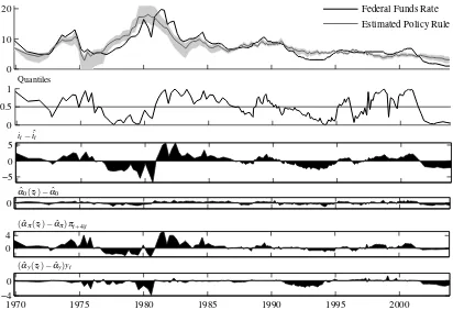
Figure 4 shows the Federal Funds Rate, the policy rule without interest rate smoothing estimated in section 5, estimated quantiles and a decomposition of deviations.14 Row 2 shows the series of estimated quantiles which is linked closely to the least squares error term shown in row 3. Row 4 shows that deviations of the IQR constant from the TSLS constant are negligible. Major deviations from the policy rule are due to persistent deviations in the inflation response shown in row 5 and the output gap response in row 6.
10I find that this minimization problem is well behaved and features a unique minimum.
11I check robustness of the results using probit, logit and nonparametric estimation methods to estimate realized quantiles.
Probit and logit estimates give similar results to the ones reported here. Nonparametric regression yields by trend similar results though showing some high frequency jumps of the estimated quantiles that might be caused by the low number of observations.
12The major advantage of the methodology used here in comparison to logit and nonparametric approaches is that the
estimated terms of the right side sum up almost exactly to the overall deviations on the left side. This is not the case when switching to other methods for estimating the quantile series. A disadvantage is that policy shocks do not show up anymore, but are absorbed in the variations of the parameters.
13The methodology is easily expanded to analyze deviations of the Federal Funds Rate from benchmark policy rules.
Deviations from Taylor’s rule can be for example decomposed as follows:it−iTaylort = [αˆ0(τt)−1] + [αˆπ(τt)−1.5]πt+4|t+ [αˆy(τt)−0.5]yt.
0 10
20 Federal Funds Rate
Estimated Policy Rule
0 0.5 1
Quantiles
−5 0 5
it−ˆit
0 ˆ
α0(τt)−αˆ0
0 4
(αˆπ(τt)−αˆπ)πt+4|t
1970 1975 1980 1985 1990 1995 2000
−4 0
[image:18.612.95.507.63.345.2](αyˆ (τt)−αyˆ )yt
Figure 4: Federal Funds Rate, Estimated Policy Rule, Quantiles and Deviation Decomposition(αi=0). Notes: Row 1 shows the Federal Funds Rate and fitted values of the estimated policy rule using TSLS together with a 95% confidence band. Row 2 shows a series of estimated quantilesτt. Row 3 shows the difference between the policy rule and the Federal Funds Rate. Rows 4-6 show the difference between estimated policy reactions and implied reactions by the policy rule. Summing up values from rows 4-6 yields row 3.
- 2002:4 (correlation coefficient: 0.42, p-value: 0.00). Thus, Federal Reserve policy responses to the output gap deviate anticyclically from a linear policy rule for the Volcker-Greenspan era. This anticyclicality together with a decreasing output gap coefficient over the conditional distribution of the interest rate implies a recession avoidance preference for the 1980 - 2002 period. The central bank reacted more to the output gap during recessions leading to a lower interest rate setting than proposed by a linear policy rule. This confirms the recession avoidance preference of the Federal Reserve found by Cukierman and Muscatelli (2008) for the Greenspan period. They estimate an in-terest rate rule with smooth-transisition models for inflation deviations from a target and the output gap to capture nonlinearities in the reaction to these two variables. Gerlach (2000) and Surico (2007) also find that the Federal Reserve responded more strongly to recessions than to expansions, but only between 1960 and 1980 and not afterwards. Gerlach (2000) uses a nonlinear policy reaction function and a HP-filtered output gap, while Surico (2007) uses the CBO output gap and squared inflation and output gap terms in a linear policy rule. The differences to my results might be due to the different methodological approach and the usage of real-time data in this study.
hidden behind the high degree of interest rate smoothing.
0 10 20
Federal Funds Rate Estimated Policy Rule
0 0.5 1
Quantiles
−4 0 4
it−ˆit
0 ˆ
α0(τt)−αˆ0
0
(αiˆ(τt)−αiˆ)it−1
0 4
(αˆπ(τt)−αˆπ)πt+4|t
1970 1975 1980 1985 1990 1995 2000
0
[image:20.612.96.509.79.373.2](αyˆ (τt)−αyˆ )yt
Figure 5:Federal Funds Rate, Estimated Policy Rule, Quantiles and Deviation Decomposition(αi6=0). Notes: see figure 4 for a description of the different graphs.
7
Conclusion
References
ADAM, K., AND R. M. BILLI (2006): “Optimal Monetary Policy under Commitment with a Zero Bound on Nominal Interest Rates,”Journal of Money, Credit, and Banking, 38(7), 1877–1905.
AMEMIYA, T. (1982): “Two Stage Least Absolute Deviations Estimators,”Econometrica, 50, 689– 711.
BLINDER, A. S. (1998): Central Banking in Theory and Practice. Cambridge, MA: MIT Press.
CHEN, L.-A.,ANDS. PORTNOY(1996): “Two-Stage Regresson Quantiles and Two-Stage Trimmed Least Squares Estimators for Structural Equation Models,”Communications in Statistics. Theory and Methods, 25(5), 1005–1032.
CHERNOZHUKOV, V.,ANDC. HANSEN(2001): “An IV Model of Quantile Treatment Effects,”
Mas-sachusetts Institute of Technology, Department of Economics, Working Paper 02-06.
(2005): “An IV Model of Quantile Treatment Effects,”Econometrica, 73(1), 245–261.
CHEVAPATRAKUL, T., T.-H. KIM, AND P. MIZEN (2009): “The Taylor Principle and Monetary Policy Approaching a Zero Bound on Nominal Rates: Quantile Regression Results for the United States and Japan,”Journal of Money, Credit and Banking, 41(8), 1705–1723.
CLARIDA, R., J. GAL´I, AND M. GERTLER (1998): “Monetary Policy Rules in Practice: Some International Evidence,”European Economic Review, 42, 1003–1067.
(2000): “Monetary Policy Rules and Macroeconomic Stability: Evidence and Some Theory,”
Quarterly Journal of Economics, 115(1), 147–180.
CUKIERMAN, A., AND A. MUSCATELLI (2008): “Nonlinear Taylor Rules and Asymmetric Prefer-ences in Central Banking: Evidence from the United Kingdom and the United States,”The B.E. Journal of Macroeconomics, 8(1).
DOLADO, J. J., R. MARIA-DOLORES, AND M. NAVEIRA (2005): “Are monetary-policy reaction functions asymmetric?: The role of nonlinearity in the Phillips curve,”European Economic Review, 49, 485 503.
FITZENBERGER, B. (1997): “The Moving Blocks Bootstrap and Robust Inference for Linear Least
Squares and Quantile Regressions,”Journal of Econometrics, 82, 235–287.
GREENSPAN, A. (1997): “Rules vs. discretionary monetary policy,” Speech at the 15th Anniversary
Conference of the Center for Economic Policy Research at Stanford University, Stanford, Califor-nia.
KATO, R.,ANDS.-I. NISHIYAMA(2005): “Optimal monetary policy when interest rates are bounded at zero,”Journal of Economic Dynamics & Control, 29, 97–133.
KOENKER, R.,ANDG. W. BASSET(1978): “Regression Quantiles,”Econometrica, 46(1), 33–50.
LEE, S. (2004): “Endogeneity in Quantile Regression Models: A Control Function Approach,”
CeMMAP Working Paper, University College London, 08/04.
MEYER, L. H., E. T. SWANSON, AND V. WIELAND (2001): “NAIRU Uncertainty and Nonlinear Policy Rules,”American Economic Review, 91(2), 226–231.
ORPHANIDES, A. (2001): “Monetary Policy Rules Based on Real-Time Data,”American Economic Review, 91, 964–985.
(2004): “Monetary Policy Rules, Macroeconomic Stability, and Inflation: A View from the Trenches,”Journal of Money, Credit and Banking, 36(2), 151–175.
ORPHANIDES, A., ANDV. WIELAND(2000): “Efficient Monetary Policy Design Near Price
Stabil-ity,”Journal of the Japanese and International Economies, 14, 327–365.
(2008): “Economic Projections and Rules of Thumb for Monetary Policy,”Federal Reserve Bank of St. Louis Review, 90(4), 307–324.
POOLE, W. (2006): “Understanding the Fed,” Speech at the Dyer County Chamber of Commerce
Annual Membership Luncheon, Dyersburg, Tenn.
POWELL, J. L. (1983): “The Asymptotic Normality of Two-Stage Least Absolute Deviations Esti-mators,”Econometrica, 51(5), 1569–1575.
SCHALING, E. (1999): “The nonlinear Phillips Curve and inflation forecast targeting,” Bank of Eng-land Working Paper No. 98.
SURICO, P. (2007): “The Feds monetary policy rule and U.S. inflation: The case of asymmetric preferences,”Journal of Economic Dynamics & Control, 31, 305–324.
TAYLOR, J. B. (1993): “Discretion versus Policy Rules in Practice,”Carnegie-Rochester Conference Series on Public Policy, 39, 195–214.
TOMOHIRO SUGO, Y. T. (2005): “The optimal monetary policy rule under the non-negativity