How better monetary statistics could have signaled the financial crisis

Munich Personal RePEc Archive

How better monetary statistics could

have signaled the financial crisis

Barnett, William A. and Chauvet, Marcelle

University of Kansas

15 June 2010

Online at

https://mpra.ub.uni-muenchen.de/24721/

- 1 -

How Better Monetary Statistics Could Have Signaled the Financial Crisis

By

William A. Barnett, University of Kansas and

Marcelle Chauvet, University of California at Riverside

June 15, 2010

ABSTRACT: This paper explores the disconnect of Federal Reserve data from index number theory. A consequence could have been the decreased systemic-risk misperceptions that contributed to excess risk taking prior to the housing bust. We find that most recessions in the past 50 years were preceded by more contractionary monetary policy than indicated by simple-sum monetary data. Divisia monetary aggregate growth rates were generally lower than simple-sum aggregate growth rates in the period preceding the Great Moderation, and higher since the mid 1980s. Monetary policy was more contractionary than likely intended before the 2001 recession and more expansionary than likely intended during the subsequent recovery.

KEY WORDS: Measurement error, monetary aggregation, Divisia index, aggregation, monetary policy, index number theory, financial crisis, great moderation, Federal Reserve.

JEL CLASSIFICATION CODE: E40, E52, E58, C43, E32

1.

Introduction

1.1. The Great Moderation and the Current Crisis

Over the past couple of decades, there has been an increasingly widely accepted view that monetary

policy had dramatically improved. In fact, some attribute this as the cause of the “Great Moderation” in

the economy‟s dynamics, by which output volatility had decreased substantially since the mid 1980s. On

Wall Street, that widely believed view was called the “Greenspan Put.” Even Lucas (2003), who has

become a major authority on the business cycle through his path-breaking publications in that area (see,

e.g., Lucas 1987), had concluded that economists should redirect their efforts towards long term fiscal

policy aimed at increasing economic growth. Since central banks were viewed as having become very

successful at damping the business cycle, he concluded that possible welfare gains from further

moderations in the business cycle were small.

It is not our intent to take a position on what the actual causes of that low volatility had been, to

argue that the Great Moderation‟s causes are gone, or that the low volatility that preceded the current

crisis will not return. Rather our objective is to investigate whether changes in monetary aggregates were

in line with intended monetary policy before and during the Great Moderation, and if there was a

significant change in the latter period that would legitimate assertions regarding a lower risk of future

- 2 -

monetary policy had significantly improved before or after the Great Moderation and, mostly important,

around recessions. We also argue that this lack of support was not factored into the decisions of many

decision makers, who had increased their leverage and risk-taking to levels now widely viewed as having

been excessive. This conclusion will be more extensively documented in Barnett (2011).

A popular media view about the recent crisis is that the firms and households that got into trouble

are to blame. According to much of the popular press and many politicians, the Wall Street professionals

and bankers are to blame for having taken excessive, self-destructive risk out of “greed.” But who are the

Wall Street professionals who decided to increase their leverage to 35:1? As is well known, they

comprise a professional elite, including some of the country‟s most brilliant financial experts. Is it

reasonable to assume that such people made foolish, self-destructive decisions out of “greed”? If so, how

should we define “greed” in economic theory, so that we can test the hypothesis? What about the

mortgage lenders at the country‟s largest banks? Were their decisions dominated by greed and

self-destructive behavior? Economic theory is not well designed to explore such hypotheses, and if the

hypotheses imply irrational behavior, how would we reconcile a model of irrational behavior with the

decisions of some of the country‟s most highly qualified experts in finance? Similarly how would one

explain the fact that the Supervision and Regulation Division of the Federal Reserve Board‟s staff ignored

the high risk loans being made by banks? Were they simply not doing their job, or perhaps did they too

believe that systemic risk had declined, so that increased risk-taking by banks was viewed to be prudent?

To find the cause of the crisis, it is necessary to look carefully at the data that produced the

impression that the business cycle had been moderated permanently to a level supporting greater risk

taking by investors and lenders. To find the causes of the “Great Moderation,” central bank policy may

be the wrong place to look. The federal funds rate has been the instrument of policy in the U.S. for over a

half century, and the Taylor rule, rather than being an innovation in policy design, is widely viewed as

fitting historic Federal Reserve behavior for a half century.1 The Great Moderation in real business cycle

1_{Although some other countries have adopted inflation targeting, Federal Reserve‟s policy innovation in recent years, if any, has}

- 3 -

volatility may have been produced by events unrelated to monetary policy, such as the growth of U. S.

productivity, improved technology and communications permitting better planning of inventories and

management, financial innovation, the rise of China as a holder of American debt and supplier of low

priced goods, perhaps permitting an expansionary monetary policy that otherwise might have been

inflationary, or even a decrease in the size and volatility of shocks, known as the “good luck” hypothesis.

This paper provides an overview of some of the data problems that produced the misperceptions of

superior monetary policy. The focus of this paper is not on what did cause the Great Moderation, but

rather on the possible causes of the misperception that there was a permanent reduction in systemic risk

associated with improved monetary policy. This paper documents the fact that the quality of Federal

Reserve data in recent years has been poor, disconnected from reputable index number theory, and

inconsistent with competent accounting principles. It is postulated that these practices could have

contributed to the misperceptions of a permanent decrease in systemic risk.

This paper‟s emphasis is on econometric results displayed in graphics. In all of the illustrations in

this paper, the source of the misperceptions is traced to data problems. We find, for example, that the

largest discrepancies between microeconomic theory-based monetary aggregate (Divisia) and simple sum

monetary aggregates occur during times of high uncertainty, such as around recessions or at the beginning

or end of high interest rate phases. In particular, the rate of growth of Divisia monetary aggregates

decrease a lot more before recessions and increase substantially more during recessions and recoveries

than simple sum aggregates. In addition, we find that the rate of growth rate of Divisia monetary

aggregates were generally lower than the rate of growth of simple sum aggregates in the period that

preceded the Great Moderation, and higher since the mid 1980s. For the recent years, this indicates, for

example, that monetary policy could have been more contractionary than intended before recessions and

more expansionary than intended during the most recent recovery after the 2001 recession. There is a

strain of thought that maintains that the current U.S. financial crisis was prompted by excessive money

creation fueling the bubbles. The process started in early 2001, when money supply was increased

substantially to minimize the economic recession that had started in March of that year. However, in

- 4 -

end in November 2001. In fact, money supply was high until mid 2004, after which it started decreasing

slowly. The argument is that the monetary expansion during this first period led to both speculation and

leveraging, especially regarding lending practices in the housing sector. This expansion is argued as

having made it possible for marginal borrowers to obtain loans with lower collateral values.

On the other hand, the Federal Reserve started increasing the target value for the federal funds rate

since June 2004. We find that the rate of growth of money supply as measured by Divisia monetary

aggregate fell substantially more than the rate of growth of simple sum monetary aggregate. Thus, the

official simple sum index could have veiled a much more contractionary policy by the Federal Reserve

than intended, which also occurred prior to most recessions in the last 50 years. For the recent period,

when money creation slowed, housing prices began to decline, leading many to own negative equity and

inducing a wave of defaults and foreclosures.

We see no reason to believe that the Federal Reserve would have as a goal to create „excessive‟

money growth. Had they known that the amount of money circulating in the economy was excessive and

could generate an asset bubble, monetary policy would have been reverted long before it did. Conversely,

we see no reason to believe that the Federal Reserve intended to have an excessive contractionary

monetary policy before the crisis. We provide evidence indicating that data problems may have misled

Federal Reserve policy to feed the bubbles with unintentionally excess liquidity and then to burst the

bubbles with excessively contractionary policy. In short, in every illustration that we provide, the motives

of the decision makers, whether private or public, were good. But the data were bad.

1.2. Overview

Barnett (1980) derived the aggregation-theoretic approach to monetary aggregation and advocated

the use of the Divisia or Fisher Ideal index with user cost prices in aggregating over monetary services.

Since then, Divisia monetary aggregates have been produced for many countries.2 But despite this vast

2 _{For example, Divisia monetary aggregates have been produced for Britain (Batchelor (1989), Drake (1992), and Belongia and}

- 5 -

amount of research, most central banks continue officially to supply the simple-sum monetary aggregates,

which have no connection with aggregation and index number theory. In contrast, the International

Monetary Fund (2008) has provided an excellent discussion of the merits of Divisia monetary

aggregation, and the Bank of England publishes them officially. The European Central Bank‟s staff uses

them in informing the Council on a quarterly basis, and the St. Louis Federal Reserve Bank provides them

for the US. The simple sum monetary aggregates have produced repeated inference errors, policy errors,

and needless paradoxes leading up to the most recent misperceptions about the source of the Great

Moderation. In this paper, we provide an overview of that history in chronological order.

We conclude with a discussion of the most recent research in this area, which introduces state-space

factor modeling into this literature. We also display the most recent puzzle regarding Federal Reserve

data on nonborrowed reserves and show that the recent behavior of that data contradicts the definition of

nonborrowed reserves. Far from resolving the earlier data problems, the Federal Reserve‟s most recent

data may be the most puzzling that the Federal Reserve has ever published.

1.3. The History

There is a vast literature on the appropriateness of aggregating over monetary asset components

using simple summation. Linear aggregation can be based on Hicksian aggregation (Hicks 1946), but that

theory only holds under the unreasonable assumption that the relative user-cost prices of the services of

individual money assets do not change over time. This condition implies that each asset is a perfect

substitute for the others within the set of components. Simple sum aggregation is an even more severe

special case of that highly restrictive linear aggregation, since simple summation requires that the

coefficients of the linear aggregator function all be the same. This, in turn, implies that the constant

user-cost prices among monetary assets be exactly equal to each other. Not only must the assets be perfect

substitutes, but must be perfect one-for-one substitutes --- i.e., must be indistinguishable assets, with one

unit of each asset being a perfect substitute for exactly one unit of each of the other assets.

In reality, financial assets provide different services, and each such asset yields its own particular

- 6 -

are not constant and are not equal across financial assets. The relative user-cost prices of U.S. monetary

assets fluctuate considerably. For example, the interest rates paid on many monetary assets are not equal

to the zero interest rate paid on currency. These observations have motivated serious concerns about the

reliability of the simple-sum aggregation method, which has been disreputable in the literature on index

number theory and aggregation theory for over a century. In addition, an increasing number of

imperfectly substitutable short-term financial assets have emerged in recent decades. Since monetary

aggregates produced from simple summation do not accurately measure the quantities of monetary

services chosen by optimizing agents, shifts in the series can be spurious and can produce erroneous

appearance of instability of structural functions containing monetary services variables.

Microeconomic aggregation theory offers an appealing alternative approach to the measurement of

money, compared to the atheoretical simple-sum method. The quantity index under the

aggregation-theoretic approach extracts and measures the income effects of changes in relative prices and is invariant

to substitution effects, which do not alter utility and thereby do not alter perceived services received. The

simple-sum index, on the other hand, does not distinguish between income and substitution effects and

thereby confounds together substitution effects with actual monetary services received. The

aggregation-theoretic monetary aggregator function, which correctly internalizes substitution effects, can be tracked

accurately by the Divisia quantity index, constructed by using expenditure shares as the component

growth-rate weights. Barnett (1978,1980) derived the formula for the user-cost price of a monetary asset,

needed in computation of the Divisia index‟s share weights, and thereby originated the Divisia monetary

aggregates. The growth rate weights resulting from this approach are different across assets, depending

on all of the quantities and interest rates in each share, and those weights can be time-varying at each

point in time. For a detailed description of the theory underlying this construction, see Barnett (1982,

1987).

The user-cost prices are foregone interest rates, with foregone interest measured as the difference

between the rate of return on a pure investment, called the benchmark asset, and the own rate of return on

the component asset. It is important to understand that the direction in which an asset‟s growth-rate

- 7 -

utility. Its shares are independent of relative prices, and hence of the interest rates within the component

user-cost prices. For other utility functions, the direction of the change in shares with a price change, or

equivalently with an interest rate change, depends upon whether the own price elasticity of demand

exceeds or is less than -1. In elementary microeconomic theory, this often overlooked phenomenon

produces the famous “diamonds versus water paradox” and is the source of most of the

misunderstandings of the Divisia monetary aggregates‟ weighting, as explained by Barnett (1983).

Several authors have studied the empirical properties of the Divisia index compared with the simple

sum index. The earliest comparisons are in Barnett (1982) and Barnett, Offenbacher, and Spindt (1984).

Barnett and Serletis (2000) collect together and reprint seminal journal articles from this literature.3

Barnett (1997) has documented the connection between the well-deserved decline in the policy-credibility

of monetary aggregates and the defects that are peculiar to simple sum aggregation.

The most recent research in this area is Barnett, Chauvet, and Tierney (2009), who compare the

different dynamics of simple-sum monetary aggregates and the Divisia indexes, not only over time, but

also over the business cycle and across high and low inflation and interest rate phases. Information about

the state of monetary growth becomes particularly relevant for policymakers, when inflation enters a

high-growth phase or the economy begins to weaken. Factor models with regime switching have been

widely used to represent business cycles (see e.g., Chauvet 1998, 2005, Chauvet and Piger 2008), but

without relationship to aggregation theory. Barnett, Chauvet, and Tierney‟s model differs from the

literature as the focus is not only on the estimated common factor, but on the idiosyncratic terms that

reflect the divergences between the simple sum and Divisia monetary aggregate in a manner relevant to

aggregation theory.

2.

Monetary Aggregation Theory

Aggregation theory and index-number theory have been used to generate official governmental data

3 _{More recent examples include Belongia (1996), Belongia and Ireland (2006), and Schunk (2001). The comprehensive survey}

- 8 -

since the 1920s. For example, the Bureau of Economic Analysis uses the Fisher ideal index in producing

the national accounts. One exception still exists. The monetary quantity aggregates and interest rate

aggregates officially supplied by many central banks are not aggregation-theoretic index numbers, but

rather are the simple unweighted sums of the component quantities and the quantity-weighted or

arithmetic averages of interest rates. The predictable consequence has been induced instability of money

demand and supply functions and a series of „puzzles‟ in the resulting applied literature. In contrast, the

Divisia monetary aggregates, originated by Barnett (1980; 1987) are derived directly from economic

index-number theory.

Data construction and measurement procedures imply the theory that can rationalize the

aggregation procedure. The assumptions implicit in the data construction procedures must be consistent

with the assumptions made in producing the models within which the data are nested. Unless the theory

is internally consistent, the data and its applications are incoherent. Without that coherence between

aggregator function structure and the econometric models within which the aggregates are embedded,

stable structure can appear to be unstable. This phenomenon has been called the „Barnett critique‟ by

Chrystal and MacDonald (1994) and in a very important recent paper by Belongia and Ireland (2010).

2.2. Aggregation Theory versus Index Number Theory

The exact aggregates of microeconomic aggregation theory depend on unknown aggregator

functions, which typically are utility, production, cost, or distance functions. Such functions must first be

econometrically estimated. Hence the resulting exact quantity and price indexes become estimator and

specification dependent. This dependency is troublesome to governmental agencies, which therefore

view aggregation theory as a research tool rather than a data construction procedure.

Statistical index-number theory, on the other hand, provides nonparametric indexes which are

computable directly from quantity and price data, without estimation of unknown parameters. Within the

literature on aggregation theory, such index numbers depend jointly on prices and quantities in two

periods, but not on unknown parameters. In a sense, index number theory trades joint dependence on

- 9 -

numbers are the Laspeyres, Paasche, Divisia, Fisher ideal, and Törnqvist indexes.

The formerly loose link between index number theory and aggregation theory was tightened, when

Diewert (1976) defined the class of second-order „superlative‟ index numbers, which track any unknown

aggregator function up to the second order. Statistical index number theory became part of

microeconomic theory, as economic aggregation theory had been for decades. Statistical index numbers

are judged by their non-parametric tracking ability to the aggregator functions of aggregation theory.

For decades, the link between statistical index-number theory and microeconomic aggregation

theory was weaker for aggregating over monetary quantities than for aggregating over other goods and

asset quantities. Once monetary assets began yielding interest, monetary assets became imperfect

substitutes for each other, and the „price‟ of monetary-asset services was no longer clearly defined. That

problem was solved by Barnett (1978; 1980) derivation of the formula for the user cost of demanded

monetary services.4

2.3. The Economic Decision

Consider a decision problem over monetary assets. The decision problem will be defined in the

simplest manner that renders the relevant literature on economic aggregation immediately applicable.5

Initially we shall assume perfect certainty.

Let m_t = (m1t, m2t, … , mnt) be the vector of real balances of monetary assets during period t, let rt

be the vector of nominal holding-period yields for monetary assets during period t, and let Rt be the one

period holding yield on the benchmark asset during period t. The benchmark asset is defined to be a pure

investment that provides no services other than its yield, Rt, so that the asset is held solely to accumulate

wealth. Thus, Rt is the maximum holding-period yield in the economy during period t.

Let yt be the real value of total budgeted expenditure on monetary services during period t. Under

4 _{Subsequently Barnett (1987) derived the formula for the user cost of supplied monetary services. A regulatory wedge can exist}

between the demand and supply-side user costs, if non-payment of interest on required reserves imposes an implicit tax on banks. Another excellent source on the supply side is Hancock (1991), who correctly produced the implicit tax on banks formula.

5 _{Our research in this paper is not dependent upon this simple decision problem, as shown by Barnett (1987), who proved that the}

- 10 -

conventional assumptions, the conversion between nominal and real expenditure on the monetary services

of one or more assets is accomplished using the true cost of living index, = (pt), on consumer

goods, where the vector of consumer goods prices is pt.6 The optimal portfolio allocation decision is:

maximize u(mt) (1)

subject to πtmt = yt,

where πt= (π1t ,…,πnt) is the vector of monetary-asset real user costs, with

πit =

1 t it t R r R   . 7 (2)

The function uis the decision maker‟s utility function, assumed to be monotonically increasing and

strictly concave.8

Let

m

the exact monetary aggregate of economic theory is the utility level associated with holding the portfolio,

and hence is the optimized value of the decision‟s objective function:

Mt = u(

m

2.4. The Divisia Index

Although equation (3) is exactly correct, it depends upon the unknown function, u. Nevertheless,

6 _{The multilateral open economy extension is available in Barnett (2007).}

7_{There is a long history regarding the “price of money.” Keynes and the classics were divided about whether it was the inflation}

rate of “the rate of interest.” The latter would be correct for noninterest bearing money in continuous time. In that case, as can be seen from equation (2), the user cost becomes Rt. More recently, Diewert (1974) acquired the formula relevant to discrete

time for noninterest bearing money, Rt /(1 + Rt). Perhaps the first to recognize the relevance of the opportunity cost, Rt– rt, for

interest bearing money was Hutt (1963, p. 92, footnote), and he advocated what later become known as the CE index derived by Rotemberg, Poterba, and Driscoll (1995). Friedman and Schwartz (1970, pp. 151-152) document many attempts by Friedman‟s students to determine the user cost formula and apply index number theory to monetary aggregation). But that work preceded the user cost derivation by Barnett and the work of Diewert () on superlative index number theory. Those attempts were not based on valid user cost formulas or modern index numbers. The best known initial attempt to use aggregation theory for monetary aggregation was by Chetty (1969). But he used an incorrect user cost formula, which unfortunately was adopted by many other economists in subsequent research in monetary aggregation. Through analogous economic reasoning, Donovan (1978) acquired the correct real user cost formula, (2). As a result of the confusion produced by the competing user cost formulas generated from economic reasoning, application to monetary aggregation was hindered until Barnett () formally derived the formula by the normal method of proof using the sequence of flow of funds identies in the relevant dynamic programming problem. Regarding that formal method of proof, see Deaton and Muellbauer (1980). Barnett‟s proof and his derivation within an internally consistent aggregation theoretic framework marked the beginning of the modern literature on monetary aggregation.

8 _{To be an admissible quantity aggregator function, the function}

umust be weakly separable within the consumer‟s complete utility function over all goods and services. Producing a reliable test for weak separability is the subject of much intensive research, most recently by Barnett and Peretti (2009). If yt were nominal, then the user cost formula would have to be nominal,

- 11 -

statistical index-number theory enables us to track Mt exactly without estimating the unknown function, u.

In continuous time, the monetary aggregate, Mt = u(

m

which solves the differential equation

*

i

log t _

_

d M d m

s

dt dt (4)

for Mt, where

*





t

m

s

y

is the i‟th asset‟s share in expenditure on the total portfolio‟s service flow.9 The dual user cost price

aggregate Πt = Π(



equation

i

log t log it

it

d d

s

dt dt









The user cost dual satisfies Fisher‟s factor reversal in continuous time:

ΠtMt = π_tmt. (6)

As a formula for aggregating over quantities of perishable consumer goods, that index was first

proposed by François Divisia (1925), with market prices and quantities of those goods used in equation

(4). In continuous time, the Divisia index, under conventional neoclassical assumptions, is exact. In

discrete time, the Törnqvist approximation is:

* *

i

log

M



log

M





s

(log

m



log

m

)

where

( )

 

it it i,t-1

1

2

s s s .

In discrete time, we often call equation (7) simply the Divisia quantity index.10 After the quantity index is

9 _{In equation (4), it is understood that the result is in continuous time, so the time subscripts are a short hand for functions of time.}

We use t to be the time period in discrete time, but the instant of time in continuous time.

10 _{Diewert (1976) defines a „superlative index number‟ to be one that is exactly correct for a quadratic approximation to the}

- 12 -

computed from (7), the user cost aggregate most commonly is computed directly from equation (6).

2.5. Risk Adjustment

Extension of index number theory to the case of risk was introduced by Barnett, Liu and Jensen

(1997), who derived the extended theory from Euler equations rather than from the perfect-certainty

first-order conditions used in the earlier index number-theory literature. Since that extension is based upon the

consumption capital-asset-pricing model (CCAPM), the extension is subject to the „equity premium

puzzle‟ of smaller-than-necessary adjustment for risk. We believe that the under-correction produced by

CCAPM results from its assumption of intertemporal blockwise strong separability of goods and services

within preferences. Barnett and Wu (2005) have extended Barnett, Liu, and Jensen‟s result to the case of

risk aversion with intertemporally non-separable tastes.11

2.6. Dual Space

User cost aggregates are duals to monetary quantity aggregates. Either implies the other uniquely.

In addition, user-cost aggregates imply the corresponding rate aggregates uniquely. The

interest-rate aggregate rt implied by the user-cost aggregate Πt is the solution for rt to the equation:

1

t t t

R

r

R





Accordingly, any monetary policy that operates through the opportunity cost of money (that is,

interest rates) has a dual policy operating through the monetary quantity aggregate, and vice versa.

Aggregation theory implies no preference for either of the two dual policy procedures or for any other

approach to policy, so long as the policy does not violate principles of aggregation theory. In their current

state-space comparisons, Barnett, Chauvet, and Tierney model in quantity space rather than the

user-cost-price or interest-rate dual spaces. Regarding policy in the dual space, see Barnett (1987) and Belongia

Fisher ideal index, rather than as a Törnqvist index. Diewert (1978) has shown that the two indexes approximate each other very well.

11 _{The Federal Reserve Bank of St. Louis Divisia database, which we use in this paper, is not risk corrected. In addition, it is not}

adjusted for differences in marginal taxation rates on different asset returns or for sweeps, and its clustering of components into

groups was not based upon tests of weak separability, but rather on the Federal Reserve‟s official clustering. The St. Louis

Federal Reserve Bank is in the process of revising its MSI database, perhaps to incorporate some of those adjustments.

- 13 -

and Ireland (2006).

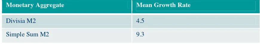
2.7. Aggregation Error and Policy Slackness

Figure 1 displays the magnitude of the aggregation error and policy slackness produced by the use

of the simple sum monetary aggregates. Suppose there are two monetary assets over which the central

bank aggregates. The quantity of each of the two component assets is y1 and y2. Suppose that the central

bank reports, as data, that the value of the simple sum monetary aggregates is Mss. The information

content of that reported variable level is contained in the fact that the two components must be

somewhere along the Figure 1 hyperplane, y1 + y2 = Mss, or more formally that the components are in the

set A:

A

= {(

y

,

y

):

y

+

y

=

M

}.

But according to equation (3), the actual value of the service flow from those asset holdings is u(y1,y2).

Consequently the information content of the information set A regarding the monetary service flow is that

the service flow is in the set E:

E

= {

u

(

y

,

y

): (

y

,

y

)



A

}.

Note that E is not a singleton. To see the magnitude of the slackness in that information, observe

from Figure 1 that if the utility level (service flow) is Mmin, then the indifference curve does touch the

hyperplane, A, at its lower right corner. Hence that indifference curve cannot rule out the Mss reported

value of the simple sum monetary aggregate, although a lower level of utility is ruled out, since

indifference curves at lower utility levels cannot touch the hyperplane, A.

Now consider the higher utility level of Mmax and its associated indifference curve in Figure 1.

Observe that that indifference curve also does have a point in common with the hyperplane, A, at the

tangency. But higher levels of utility are ruled out, since their indifference curves cannot touch the

hyperplane, A. Hence the information about the monetary service flow, provided by the reported value of

the simple sum aggregate, Mss, is the interval

E = [Mmin,Mmax].

The supply side aggregation is analogous, but the lines of constant supplied service flow for

- 14 -

3.

The History of Thought on Monetary Aggregation

The fields of aggregation and index number theory have a long history. The first book to put

together the properties of all of the available index numbers in a systematic manner was the famous Irving

Fisher (1922). He made it clear in that book that the simple sum and arithmetic average indexes are the

worst known indexes. On p. 29 of that book he wrote:

“The simple arithmetic average is put first merely because it naturally comes first to the reader‟s mind, being

the most common form of average. In fields other than index numbers it is often the best form of average to

use. But we shall see that the simple arithmetic average produces one of the very worst of index numbers,

and if this book has no other effect than to lead to the total abandonment of the simple arithmetic type if index

number, it will have served a useful purpose.”

On p. 361 Fisher wrote:

“The simple arithmetic should not be used under any circumstances, being always biased and usually

freakish as well. Nor should the simple aggregative ever be used; in fact this is even less reliable.”

The simple sum monetary aggregates published by the Federal Reserve are produced from the

“simple aggregative” quantity index.12

Indeed data-producing agencies and data-producing newspapers

switched to reputable index numbers, following the appearance of Fisher‟s book. But there was one

exception: the world‟s central banks, which produced their monetary aggregates as simple sums. While

the implicit assumption of perfect substitutability in identical ratios might have made sense during the

first half of the 20th century, that assumption became unreasonable, as interest-bearing substitutes for

currency were introduced by financial intermediaries, such as interest bearing checking and saving

accounts.

Nevertheless, the nature of the problem was understood by Friedman and Schwartz (1970,

12 _{While Fisher‟s primary concern was price index numbers, any price index formula has an analogous quantity index number}

- 15 -

151-152), who wrote the following:

“The [simple summation] procedure is a very special case of the more general approach. In brief, the general

approach consists of regarding each asset as a joint product having different degrees of „moneyness,‟ and

defining the quantity of money as the weighted sum of the aggregated value of all assets…. We conjecture

that this approach deserves and will get much more attention than it has so far received.”

More recently, subsequent to Barnett‟s derivation of the Divisia monetary aggregates, Lucas (2000,

p. 270) wrote:

“I share the widely held opinion that M1 is too narrow an aggregate for this period [the 1990s], and I think

that the Divisia approach offers much the best prospects for resolving this difficulty.”

4.

The 1960s and 1970s

Having surveyed the theory and some of the relevant historical background, we now provide some

key results. We organize them chronologically, to make the evolution of views clear. We first provide

results for the 1960s and 1970s. The formal econometric source of the graphical results in this section,

along with further modeling and inference details, can be found in Barnett, Offenbacher, and Spindt

(1984) and Barnett (1982).

Demand and supply of money functions were fundamental to macroeconomics and to central bank

policy until the 1970s, when questions began to arise about the stability of those functions. It was

common for general equilibrium models to determine real values and relative prices, and for the demand

and supply for money to determine the price level and thereby nominal values. But it was believed that

something went wrong in the 1970s. In Figure 2, observe the behavior of the velocity of M3 and M3+

(later called L), which were the two broad aggregates often emphasized in that literature. For the demand

for money function to have the correct sign for its interest elasticity (better modeled as user-cost price

elasticity), velocity should move in the same direction as nominal interest rates.

Figure 3 provides an interest rate during the same time period. Note that while nominal interest

rates were increasing during the growing inflation of that decade, the velocity of the simple sum monetary

- 16 -

not exist, when the data were produced from index number theory.

Much of the concern in the 1970s was focused on 1974, when it was believed that there was a sharp

structural shift in money markets. Figure 4 displays a source of that concern. As is evident from this

figure – which plots velocity against a bond rate, rather than against time –– there appears to be a

dramatic shift downwards in that velocity function in 1974. But observe that this result was acquired

using simple sum M3. Figure 5 displays the same cross plot of velocity against an interest rate, but with

M3 computed as its Divisia index. Observe that velocity no longer is constant, either before or after

1974. But there is no structural shift.

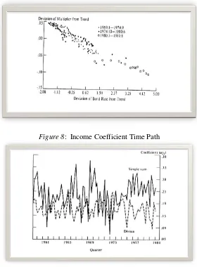
There were analogous concerns about the supply side of money markets. The reason is evident

from Figure 6, which plots the base multiplier against a bond rate‟s deviation from trend. The base

multiplier is the ratio of a monetary aggregate to the monetary base. In this case, the monetary aggregate

is again simple sum M3. Observe the dramatic structural shift. Prior to 1974, the function was a

parabola. After 1974 the function is an intersecting straight line. But again this puzzle was produced by

the simple-sum monetary aggregate. In Figure 7, the same plot is provided, but with the monetary

aggregate changed to Divisia M2. The structural shift is gone.

The econometric methods of investigating these concerns at the time were commonly based on the

use of the Goldfeld (1973) demand for money function, which was the standard specification used by the

Federal Reserve System. The equation was a linear regression of a monetary aggregate on national

income, a regulated interest rate, and an unregulated interest rate. It was widely believed that the function

had become unstable in the 1970s.

Swamy and Tinsley (1980), at the Federal Reserve Board in Washington, DC, had produced a

stochastic coefficients approach to estimating a linear equation. The result was an estimated stochastic

process for each coefficient. The approach permitted testing the null hypothesis that all of the stochastic

processes are constant. Swamy estimated the processes for the model‟s three coefficients at the Federal

Reserve Board with quarterly data from 1959:2 – 1980:4, and the econometric results were published by

Barnett, Offenbacher, and Spindt (1984). The realizations of the three coefficient processes are displayed

- 17 -

simple sum M2. The dotted line is the realization, when the monetary aggregate is measured by the

Divisia index. The instability of the coefficient is very clear, when the monetary aggregate is simple sum;

but the processes look like noise around a constant, when the monetary aggregate is Divisia. The

statistical test could not reject constancy (i.e., stability of the demand for money function), when Divisia

was used. But stability was rejected, when the monetary aggregate was simple sum.

5.

The Monetarist Experiment: November 1979

–

November 1982

Following the inflationary 1970s, Paul Volcker, as Chairman of the Federal Reserve Board, decided

to bring inflation under control by decreasing the rate of growth of the money supply, with the instrument

of policy being changed from the federal funds rate to nonborrowed reserves. The period, November

1979 –November 1982, during which that policy was applied, was called the “Monetarist Experiment.”

The policy succeeded in ending the escalating inflation of the 1970s, but was followed by an unintended

recession. The Federal Reserve had decided that the existence of widespread 3-year negotiated wage

contracts precluded a sudden decrease in the money supply growth rate to the intended long run growth

rate. The decision was to decrease from the high double-digit growth rates to about 10% per year and

then gradually decrease towards the intended long run growth rate to avoid inducing a recession.

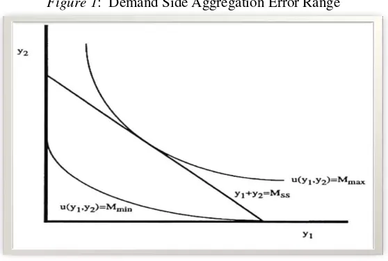
Figure 11 and Table 1 reveal the cause of the unintended recession. As is displayed in Figure 11

for the M3 levels of aggregation, the rate of growth of the Divisia monetary aggregate was substantially

less than the rate of growth of the official simple-sum-aggregate intermediate targets. As Table 1

summarizes, the simple sum aggregate growth rates were at the intended levels, but the Divisia growth

rates were half as large, producing a negative shock of substantially greater magnitude than intended. For

computational details, see Barnett (1984). A recession followed.

6.

End of the Monetarist Experiment: 1983 - 1984

Following the end of the Monetarist Experiment and the unintended recession that followed, Milton

Friedman became very vocal with his prediction that there had just been a huge surge in the growth rate

- 18 -

inflation. He further predicted that there would subsequently be an overreaction by the Federal Reserve,

plunging the economy back down into a recession. He published this view repeatedly in the media in

various magazines and newspapers, with the most visible being his Newsweekarticle, “A Case of Bad

Good News,” which appeared on p. 84 on September 26, 1983. We have excerpted some of the sentences

from that Newsweek article below:

“The monetary explosion from July 1982 to July 1983 leaves no satisfactory way out of our present situation.

The Fed‟s stepping on the brakes will appear to have no immediate effect. Rapid recovery will continue under

the impetus of earlier monetary growth. With its historical shortsightedness, the Fed will be tempted to step

still harder on the brake – just as the failure of rapid monetary growth in late 1982 to generate immediate

recovery led it to keep its collective foot on the accelerator much too long. The result is bound to be renewed

stagflation – recession accompanied by rising inflation and high interest rates... The only real uncertainty is

when the recession will begin.”

But on exactly the same day, September 26, 1983, William Barnett published a very different view

in his article, “What Explosion?” on p. 196 ofForbes magazine. The following is an excerpt of some of

the sentences from that article:

“People have been panicking unnecessarily about money supply growth this year. The new bank money

funds and the super NOW accounts have been sucking in money that was formerly held in other forms, and

other types of asset shuffling also have occurred. But the Divisia aggregates are rising at a rate not much

different from last year‟s... the „apparent explosion‟ can be viewed as a statistical blip.”

Milton Friedman would not have taken such a strong position without reason. You can see the

reason from Figure 12. The percentage growth rates in that figure are divided by 10, so should be

multiplied by 10 to acquire the actual growth rates. Notice the large spike in growth rate, which rises to

near 30% per year. But that solid line is produced from simple sum M2, which was greatly

overweighting the sudden new availability of super-NOW accounts and money market deposit accounts.

There was no spike in the Divisia monetary aggregate, represented by the dashed line.

If the huge surge in the money supply had happened, then inflation would surely have followed,

- 19 -

there was no inflationary surge and no subsequent recession.

7.

The Rise of Risk Adjustment Concerns: 1984 - 1993

The exact monetary quantity aggregator function,

m

= u(

m

), can be tracked very accurately

by the Divisia monetary aggregate,

m

, since its tracking ability is known under perfect certainty.

However, when nominal interest rates are uncertain, the Divisia monetary aggregate's tracking

ability is somewhat compromised. That compromise is eliminated by using the extended Divisia

monetary aggregate under risk derived by Barnett, Liu, and Jensen (1997). Let

m

denote the

extended “generalized” Divisia monetary aggregate. The only difference between m

and m

is

the risk-adjusted user cost formula used to compute the prices in the generalized Divisia index

formula.

Let



denote the generalized user cost of monetary asset

i

. Under CCAPM (consumptions

capital asset pricing) assumptions, Barnett, Liu, and Jensen (1997) prove that

it G it e it

=

+







where

e t t it t t

= E ( R - R ) E (1+ R )



and

= E (1+ R ) E (1+ R )

Cov( R , T C ) T C

-Cov( R , T C ) T C ,



where

).

,

(

c

m

F

E

=

T







Barnett, Liu, and Jensen (1997) show that the values of

φ

determine the risk premia in interest

- 20 -

Using that extension, Barnett and Xu (1998) demonstrated that velocity will change, if the

variance of an interest rate stochastic process changes. Hence the variation in the variance of an

interest rate ARCH or GARCH stochastic process cannot be ignored in modelling monetary

velocity. By calibrating a stochastic dynamic general equilibrium model, Barnett and Xu (1998)

showed that the usual computation of the velocity function will be unstable, when interest rates

exhibit stochastic volatility. But when the CCAPM adjusted variables above are used, so that the

variation in variance is not ignored, velocity is stabilized.

Figure 13 displays the simulated slope coefficient for the velocity function, treated as a

function of the exact interest rate aggregate, but without risk adjustment. All functions in the

model are stable, by construction. Series 1 was produced with the least stochastic volatility in the

interest rate stochastic process, series 2 with greater variation in variance, and series 3 with even

more stochastic volatility. Note that the velocity function slope appears to be increasingly

unstable, as stochastic volatility increases. By the model‟s construction, the slope of the velocity

function is constant, if the CCAPM risk adjustment is used. In addition, with real economic data,

Barnett and Xu (1998) showed that the evidence of velocity instability is partially explained by

overlooking the variation in the variance of interest rates over time.

Subsequently Barnett and Wu (2005) found that the explanatory power of the risk adjustment

increases, if the assumption of intertemporal separability of the intertemporal utility function, T, is

weakened. The reason is the same as a source of the well known equity premium puzzle, by which

CCAPM under intertemporal separability under-corrects for risk.

The Divisia index tracks the aggregator function, which measures service flow. But for

some purposes, the economic capital stock, computed from the discounted expected future

service flow, is relevant, especially when investigating wealth effects of policy. The economic

- 21 -

immediately from the manner in which monetary assets are found to enter the derived wealth

constraint, (2.3). As a result, the formula for the economic stock of money under perfect

foresight is

1 1

(1 )

n

s s is

t is

s t i s s

p p r

V m          _           ,

where the true cost of living index on consumer goods is

=

(

p

), with the vector of

consumer goods prices being

p

, and where the discount rate for period

s

is

1 1 (1 ) s s u u t

for s t

R for s t

       _{  }   .

The CCAPM extension of the economic capital stock formula to risk is available from Barnett,

Chae, and Keating (2006).

During the late 1980s and early 1990s, there was increasing concern about substitution of

monetary assets within the monetary aggregates (especially money market mutual funds) with

stock and bond mutual funds, which are not within the monetary aggregates. The Federal

Reserve Board staff considered the possibility of incorporating stock and bond mutual funds into

the monetary aggregates. Barnett and Zhou (1994a) used the formulas above to investigate the

problem. They produced the figures that we reproduce below as Figures 14 and 15. The dotted

line is the simple sum monetary aggregate, which Barnett (2000) proved is equal to the sum of

economic capital stock of money,

V

, and the discounted expected investment return from the

components.

Computation of

V

requires modeling expectations. In that early paper, Barnett and Zhou

(1994a) used martingale expectations rather than the more recent approach of Barnett, Chae, and

Keating, using VAR forecasting. When martingale expectations are used, the index is called CE.

Since the economic capital stock of money,

V

, is what is relevant to macroeconomic theory, we

- 22 -

parallel time paths, so that the growth rate is about the same in either. That figure is for M2+,

which was the Federal Reserve Board staff‟s proposed extended aggregate, adding

stock and

bond mutual funds to M2. But note that in Figure 14, the gap between the two graphs is

decreasing, producing a slower rate of growth for the simple sum aggregate than for the

economic stock of money.

The gap between the two lines is the amount motivated by investment yield. Clearly those gaps had

been growing. But it is precisely that gap which does not measure monetary services. By adding the

value of stock and bond mutual funds into Figure 14 to get Figure 15, the growth rate error of the simple sum aggregate is offset by adding in an increasing amount of assets providing nonmonetary services.

Rather than trying to stabilize the error gap by adding in more and more nonmonetary services,

the correct solution would be to remove the entire error gap by using the solid line in Figure 14,

which measures the actual economic capital stock of money.

8.

The Y2K Computer Bug: 1999-2000

The next major concern about monetary aggregates and monetary policy arose at the end of

1999. In particular, the financial press became highly critical of the Federal Reserve for what

was perceived by those commentators to be a large, inflationary surge in the monetary base. The

reason is clear from Figure 16. But in fact there was no valid reason for concern, since the cause

was again a problem with the data.

The monetary base is the sum of currency plus bank reserves. Currency is dollar for dollar

pure money, while reserves back deposits in an amount that is a multiple of the reserves. Hence

as a measure of monetary services, the monetary base is severely defective, even though it is a

correct measure of “outside money.” At the end of 1999, there was the so

-called Y2K computer

bug, which was expected to cause temporary problems with computers throughout the world,

including at banks. Consequently many depositors withdrew funds from their checking accounts

- 23 -

currency demand, the decrease in deposits produced a smaller decline in reserves, because of the

multiplier from reserves to deposits. The result was a surge in the monetary base, even though

the cause was a temporary dollar-for-dollar transfer of funds from demand deposits to cash,

having little effect on economic liquidity. Once the computer bug was resolved, people put the

withdrawn cash back into deposits, as is seen from Figure 17.

9.

The Supply Side

While much of the concern in this literature has been about the demand for money, there is

a parallel literature about the supply of money by financial intermediaries. Regarding the

aggregation theoretic approach, see Barnett and Hahm (1994) and Barnett and Zhou (1994b). It

should be observed that the demand-side Divisia monetary aggregate, measuring perceived

service flows received by financial asset holders, can be slightly different from the supply-side

Divisia monetary aggregate, measuring service flows produced by financial intermediaries. The

reason is the regulatory wedge resulting from non-interest-bearing required reserves. That

wedge produces a difference between demand side and supply-side user-cost prices and thereby

can produce a small difference between the demand side and supply side Divisia aggregates.

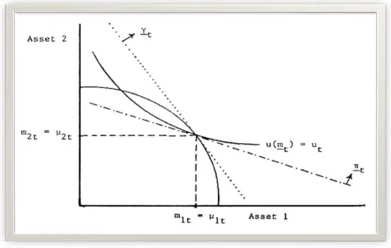
When there are no required reserves and hence no regulatory wedge, the general

equilibrium looks like Figure 18, with the usual separating hyperplane determining the user cost

prices, which are the same on both sides of the market. The production possibility surface

between deposit types 1 and 2 is for a financial intermediary, while the indifference curve is for a

depositor allocating funds over the two asset types. In equilibrium, the quantity of asset

i

demanded, m

, is equal to the quantity supplied, μ

, and the slope of the separating hyperplane

determines the relative user costs on the demand side, π

, which are equal to those on the supply

side, γ

.

- 24 -

But when noninterest-bearing required reserves exist, the foregone investment return to banks is

an implicit tax on banks and produces a regulatory wedge between the demand and supply side.

It was shown by Barnett (1987) that under those circumstances, the user cost of supplied

financial services by banks is not equal to the demand price, (2), but rather is

γ

=

(1

)

1

it t it t

k R

r

R







,

where

k

is the required reserve ratio for account type

i

, r

again is the interest rate paid on

deposit type

i

, and now the bank‟s benchmark rate, R

, is its loan rate. Note that this supply-side

user cost is equal to the demand-side formula, (2), when

k

= 0, if the depositor‟s benchmark rate

is equal to the bank‟s loan rate, as in classical macroeconomics, in which there is one pure

investment rate of return.

The resulting general equilibrium diagram, with the regulatory wedge, is displayed in Figure

19. Notice that one tangency determines the supply-side prices, while the other tangency produces

the demand-

side prices, with the angle between the two straight lines being the “regulatory

wedge.” Observe

that the demand equals the supply for each of the two component assets.

Although the component demands and supplies are equal to each other, the failure of

tangency between the production possibility curve and the indifference curve can result in a wedge

between the growth rates of aggregate demand and supply services, as reflected in the fact that the

user cost prices in the Divisia index are not the same in the demand and the supply side aggregates.

To determine whether this wedge might provide a reason to compute and track the Divisia

monetary supply aggregate as well as the more common demand-side Divisia monetary aggregate,

Barnett, Hinich, and Weber (1986) conducted a detailed spectral analysis in the frequency domain.

Figure 20 displays the squared coherence between the demand and supply side Divisia

13 _{An excellent source on the supply side is Hancock (1985a,1985b,1991), who independently acquired many of the same results}

- 25 -

monetary aggregates, where coherence measures correlation as a function of frequency. The figure

provides those plots at three levels of aggregation. Note that the correlation usually exceeds 95%

for all three levels of aggregation at all frequencies, but the coherence begins to decline at very

high frequencies (i.e., very short cycle periods in months). Hence the difference between the

demand and supply side monetary aggregates is relevant only in modelling very short run

phenomena.

To put this into context, we displays plots in the time domain for simple-sum M3, the

supply-side M3 Divisia index (SDM3), and the demand-supply-side M3 Divisia index (DDM3) over the same

time period used in producing the frequency domain comparisons. See Figure 21 for those plots.

Notice that it takes over a decade for the difference between the demand side and supply side

Divisia index to get wider than a pencil point, but the divergence between simple sum and either of

the two Divisia aggregates begins immediately and is cumulative. In short, the error in using the

simple-sum monetary aggregates is overwhelmingly greater than the usually entirely negligible

difference between the demand and supply side Divisia monetary aggregates. Furthermore, in

recent years reserve requirements have been low and largely offset by sweeps. In addition, the

Federal Reserve recently began paying interest on required reserves, although not necessarily at

bank‟s full loan rate. The differen

ce between the demand and supply side Divisia monetary

aggregates now is much smaller than during the time period displayed in Figures 20 and 21.

10.

The Great Moderation

The most recent research on the comparison of microeconomic aggregated-based Divisia

and the simple sum monetary aggregates is Barnett, Chauvet, and Tierney (2009). The paper

proposes a latent factor Markov switching approach that separates out common dynamics in

monetary aggregates from their idiosyncratic movements. The dynamic factor measures the

- 26 -

captures movements peculiar to each index. The approach is used to provide pairwise

comparisons of Divisia versus simple-sum monetary aggregates quarterly from 1960:2 to 2005:4.

In that paper, they introduced the connection between the state-space time-series approach to

assessing measurement error and the aggregation theoretic concept, with emphasis upon the

relevancy to monetary aggregation and monetary policy.

10.1. The Model

Let

Y

be the

n

x 1 vector of monetary indexes, where

n

is the number of monetary indexes

in the model:

Yt = Ft+t+vt, (8)

where



= 1

–

L and L is the lag operator. Changes in the monetary aggregates,



Y

, are

modeled as a function of a scalar unobservable factor that summarizes their commonalities,



F

;

an idiosyncratic component

n

x 1 vector, which captures the movements peculiar to each index,

v

; and a scalar potential time trend



. The factor loadings,



, measure the sensitivity of the

series to the dynamic factor,



F

. Both the dynamic factor and the idiosyncratic terms follow

autoregressive processes:

Ft =αS_t + (L)Ft-1t t~N(0, σ2), (9)

vt= h t

S

Γ +d(L)vt-1+t, t~ i.i.d. N(0,      (10)

where



is the common shock to the latent dynamic factor, and



are the measurement errors. In

order to capture potential nonlinearities across different monetary regimes, the intercept of the

monetary factor switches regimes according to a Markov variable,

S

, where



+





t

S

,

and

= 0, 1. That is, monetary indexes can either be in an expansionary regime, where the

mean growth rate of money is positive (

= 1), or in a contractionary phase with a lower or

negative mean growth rate (

= 0).

- 27 -

Markov processes, by allowing their drift terms,



t

S

Γ

, to switch between regimes. For example,

in the case of two monetary indexes,

n

= 2, there will be two idiosyncratic terms, each one

following an independent Markov process

and



t

S

, where

= 0, 1 and



t

S

= 0, 1. Notice

that we do not constraint the Markov variables

,



t

S

, and



to be dependent of each other,

but allow them instead to move according to their own dynamics. In fact, there is no reason to

expect that the idiosyncratic terms would move in a similar manner to each other or to the

dynamic factor, since by construction they represent movements peculiar to each index not

captured by the common factor.

The switches from one state to another is determined by the transition probabilities of the first-order

two-state Markov processes, k

ij

p = P( k t

S =j| k t

S1= i), where 1 01,

1

0p ,i,j ,

j k

ij  



identifying the Markov processes for the dynamic factor and the two idiosyncratic terms, respectively.

The model separates out the common signal underlying the monetary aggregates from

individual variations in each of the indexes. The dynamic factor captures simultaneous

downturns and upturns in money growth indexes. On the other hand, if only one of the variables

declines, e.g. M1, this would not characterize a general monetary contraction in the model and

would be captured by the M1 idiosyncratic term. A general monetary contraction (expansion)

will occur when all

n

variables decrease (increase) at about the same time. That is,



and

v

are

assumed to be mutually independent at all leads and lags for all

n

variables, and

d

(L) is diagonal.

The dynamic factor is the outcome of averaging out the discrete states. Although the

n

monetary

indexes represent different measurements of money, the estimated dynamic factor is a nonlinear

combination of them, representing broader movements in monetary aggregates in the U.S. On

the other hand, once a contraction or expansion is clearly under way, the idiosyncratic term for a

particular aggregate can be highly informative near a turning point.