The Analytical Expressions for Computing the Minimum Distance between a Point and a Torus

(1)

http://dx.doi.org/10.4236/jcc.2016.44011

How to cite this paper: Li, X.W., Hou, L.K., Liang, J., Wu, Z.N., Wang, L. and Yue, C.G. (2016) The Analytical Expressions for Computing the Minimum Distance between a Point and a Torus. Journal of Computer and Communications, 4, 125-133. http://dx.doi.org/10.4236/jcc.2016.44011

The Analytical Expressions for Computing

the Minimum Distance between a

Point and a Torus

Xiaowu Li1*_{, Linke Hou}2*_{, Juan Liang}3*_{, Zhinan Wu}4_{, Lin Wang}1_{, Chunguang Yue}1*

1_{College of Information Engineering, Guizhou Minzu University, Guiyang, China} 2_{Center for Economic Research, Shandong University, Jinan, China}

3_{Department of Science, Taiyuan Institute of Technology, Taiyuan, China}

4_{School of Mathematics and Computer Science, Yichun University, Yichun, China}

Received 2 March 2016; accepted 19 April 2016; published 22 April 2016

This work is licensed under the Creative Commons Attribution International License (CC BY).

http://creativecommons.org/licenses/by/4.0/

Abstract

In this paper, we present the analytical expressions for computing the minimum distance between a point and a torus, which is called the orthogonal projection point problem. If the test point is on the outside of the torus and the test point is at the center axis of the torus, we present that the or-thogonal projection point set is a circle perpendicular to the center axis of the torus; if not, the analytical expression for the orthogonal projection point problem is also given. Furthermore, if the test point is in the inside of the torus, we also give the corresponding analytical expression for orthogonal projection point for two cases.

Keywords

Point Projection, Center Axis of the Torus, Major Planar Circle, Minor Planar Circle, Intersection

1. Introduction

In this paper, we discuss how to compute the minimum distance between a point and a spatial parametric surface and to return the nearest point on the surface as well as its corresponding parameter, which is also called the point projection problem (the point inversion problem) of a spatial parametric surface. It is very interesting for this problem due to its importance in geometric modeling, computer graphics and computer vision [1]. Both

(2)

projection and inversion are essential for interactively selecting surfaces [1] [2], for the surface fitting problem [1] [2], for the reconstructing surfaces problem [3]-[5]. It is also a key issue in the ICP iterative close for construction and rendering of solid models with boundary representation, projecting of a space curve onto a surface for curve surface design [6]. Many algorithms have been developed by using various techniques including turning into solving a root problem of a polynomial equations, geometric methods, subdivision methods, circular clipping algorithm. For more details, see [1]-[23] and the references therein.

In the various methods mentioned above, all the iterative processes can produce one iterative solution. Different from the above methods, we consider the special situation which the test point have countless corresponding solutions for the orthogonal projection problem. We present the analytical expression for computing the minimum distance between a point and a torus. If the test point is on the outside of the torus and the test point is at the center axis of the the torus, we know that the orthogonal projection point set is a circle which is perpendicular to the center axis of the torus; If not, the analytical expression for the orthogonal projection point problem is also given. In addition, if the test point is in the inside of the torus and is on the major planar circle, then the corresponding analytical expression for orthogonal projection point set is minor planar circle. Moreover, if the test point is in the inside of the torus and is not on the major planar circle, we also present the corresponding analytical expression for orthogonal projection point of the test point.

2. Computing the Minimum Distance between a Point and a Torus

2.1. Test Point Being on the Outside of the Torus

The torus Γ can be defined as

(

)

2

2 2 2 2

x +y −R +z =r (1) in R3, where R>r. In this subsection, we suppose that test point

(

x y z0, 0, 0

)

is on the outside of the torus,

namely,

(

)

2

2 2 2 2

0 0 0

onto a torus surface Γ can be

done as follows. Major planar circle is defined as

2 2 2

, 0.

x y R

z

 + =

 =

 (2)

Assume that the coordinates of arbitrary point of major planar circle is

(

x y1, 1, 0

)

which is satisfied

2 2 2

1 1

1

,

0.

x y R

z

 + =



 ₌

 (3)

)

1

0 0

,

, 0 1

.

x x t

y y t t

z z z t

= ⋅ 

 = ⋅ < <



 = − ⋅ 

(4)

From (1) and (4), we get that the corresponding parameter value of intersection of parametric equation for the

line segment L1 and the torus Γ is

2 2 0

1 r

t

R z

= −

+ . Then the intersection of the line segment L1 and the

(3)

1 1 1 1 0

2 2 2 2 2 2

0 0 0

, , ,

r r r

x x y y z

R z R z R z

 

 − − 

 ₊ ₊ ₊ 

 

or another form

1 1 ₂ ₂

0

1 1 ₂ ₂

0

2 2 0

,

.

r

x x x

R z

r

y y y

R z

r

z z

R z

  = −

 +

  = − 

+ 

  =

 ₊



(5)

By (3) and (5), we obtain

2

2 2 2

2 2

0

2 2

0

1 ,

.

r

x y R

R z

r

z z

R z

 _ _

 ₊ ₌ _ ₋ _

  

 _ + _

 

= 

+ 

(6)

In the case of the test point being at the center axis of the torus, Formula (6) indicates that the corresponding orthogonal projection point set of the test point is a circle which parallels to major planar circle (seeFigure 1).

(

x y z0, 0, 0

)

and torus Γ

according to this idea. We deduce that the general plane equation Ω0 passing through the z-axis is

0 0 0.

[image:3.595.65.536.77.349.2] [image:3.595.213.412.529.687.2]

y x−x y= (7) From (2) and (7), we obtain that the corresponding intersection of the plane Ω0 and major planar circle of

(4)

the torus is 0 0

2 2 2 2

0 0 0 0

, , 0

R x R y

x y x y

 _⋅ _⋅ 

 

 ₊ ₊ 

  and

0 0

2 2 2 2

0 0 0 0

, , 0

R x Ry

x y x y

 _⋅ 

− − 

 ₊ ₊ 

 . If the intersection of the plane 0 Ω

and major planar circle of the torus is 0 0

2 2 2 2

0 0 0 0

, , 0

R x R y

x y x y

 _⋅ _⋅ 

 

 ₊ ₊ 

 

, then the corresponding vector between this

intersection and test point

(

x y z0, 0, 0

)

is

0 0

0 0 0

2 2 2 2

0 0 0 0

, ,

R x R y

x y z

x y x y

 _⋅ _⋅ 

 

= − −

 ₊ ₊ 

 

n . Furthermore the parameter

equation of the line segment L2 determined by the intersection

0 0

2 2 2 2

0 0 0 0

, , 0

R x R y

x y x y

 _⋅ _⋅ 

 

 ₊ ₊ 

  and test point

(

x y z0, 0, 0

)

is

(

)

0 0

0

2 2 2 2

0 0 0 0

0 0

0

2 2 2 2

0 0 0 0

0

,

0 1

,

.

R x R x

x x t

x y x y

t

R y R y

y y t

x y x y

z z t

 _⋅  _⋅ 

 = + − ⋅

 

 + _ + _

 _{< <}

   _⋅ _⋅    = + − ⋅    + _ + _  = ⋅  (8)

And because the intersections of the torus Γ and the plane Ω0 is the following first minor planar circle Ψ0

(

)

2

2 2 2 2

0 0

,

0,

x y R z r

y x x y

 ₊ ₋ ₊ ₌    − =  (9)

by (8) and (9), the corresponding parameter value of intersection of the line segment L2 and the minor planar

circle Ψ0 is

(

)

2

2 2 2

0 0 0

r t

x y R z

=

+ − +

. Substituting this parameter value into (8), we obtain the intersection

(

x w y w z w0 0, 0 0, 0 1

)

where

(

)

0

2 2 2 2 2

2 2 2

0 0 0 0

0 0 0

1

R R r

w

x y x y

x y R z

 

 

= + − ⋅

 

+ _ + _ ₊ ₋ ₊ and

(

)

1 ₂

2 2 2

0 0 0

r w

x y R z

=

+ − +

. If the intersection of the plane Ω0 and the major planar circle of the torus is

0 0

2 2 2 2

0 0 0 0

, , 0

R x R y

x y x y

 _⋅ _⋅ 

− − 

 ₊ ₊ 

 

, then the corresponding vector between this intersection 0 0

2 2 2 2

0 0 0 0

, , 0

R x R y

x y x y

 _⋅ _⋅ 

− − 

 ₊ ₊ 

 

and the test point

(

x y z0, 0, 0

)

is

0 0

0 0 0

2 2 2 2

0 0 0 0

, ,

R x R y

x y z

x y x y

 _⋅ _⋅ 

 

= + +

 ₊ ₊ 

 

n . Furthermore the parameter equation

of the line segment L3 determined by the intersection

0 0

2 2 2 2

0 0 0 0

, , 0

R x R y

x y x y

 _⋅ _⋅ 

− − 

 ₊ ₊ 

 

and the test point

(5)

(

)

0 0

0

2 2 2 2

0 0 0 0

0 0

0

2 2 2 2

0 0 0 0

0

0 1

R x R x

x x t

x y x y

t

R y R y

y y t

x y x y

z z t

 _⋅  _⋅ 

 = − + + ⋅

 

 ₊ _ ₊ _

 _{< <}

   _⋅ _⋅    = − + + ⋅    + _ + _  = ⋅  (10)

Because the intersections of the torus Γ and the plane Ω₀ is the following second minor planar circle Ψ₁

(

)

2

2 2 2 2

0 0

,

0,

x y R z r

y x x y

 ₊ ₋ ₊ ₌    ₋ ₌  (11)

from (10) and (11), the intersection parameter of the line segment L3 and the second minor planar circle Ψ1

is

(

)

2

2 2 2

0 0 0

r t

x y R z

=

+ + +

. Substituting this parameter value into (10), we get the second intersection

(

x w y w z w0 2, 0 2, 0 3

)

of the segment line L3 and the torus Γ where

(

)

2

2 2 2 2 2

2 2 2

0 0 0 0

0 0 0

1

R R r

w

x y x y

x y R z

 

 

= − + + ⋅

 

+ _ + _ ₊ ₊ ₊ and 3

(

)

2

2 2 2

0 0 0

r w

x y R z

=

+ + +

.

is at the outside of the torus Γ, so

(

)

2

2 2 2

0 0 0

x +y −R +z >r. It is easy to know that

(

)

2

2 2 2

0 0 0

x +y +R +z >r. From the two inequalities, we get

(

)

(

)

2 2

0 0 ₂ ₂

2 2 2 2 2 2

0 0 0 0 0 0

2

4R x y 1 r 0.

x y R z x y R z

 

 

+ − >

 

+ − + + + + +

 

 

And because of

(

)

(

)

(

)

(

)

(

) (

)

(

) (

)

2 2

0 0 ₂ ₂

2 2 2 2 2 2

0 0 0 0 0 0

2 2

2 2 2 2 2 2 2 2

0 0 0 0 0 0 0 0

2 2 2 2 2 2

0 2 0 0 2 0 0 3 0 0 1 0 0 1 0 0 1 0

2

4 1

4 2 2

,

r

R x y

x y R z x y R z

R x y r x y R z r x y R z

x w x y w y z w z x w x y w y z w z

      + −  ₊ ₋ ₊ ₊ ₊ ₊ ₊      = + − + + + + + − + = − + − + − − − + − + −

so it exists inequality relationship

(

) (

2

) (

2

)

2

(

) (

2

) (

2

)

2

0 2 0 0 2 0 0 3 0 0 1 0 0 1 0 0 1 0 .

x w −x + y w −y + z w −z > x w −x + y w −y + z w −z

This demonstrates that the distance between the second intersection and the test point is longer than the distance between the first intersection and the test point. Thus the distance between the intersection

(6)

[image:6.595.201.429.85.284.2]

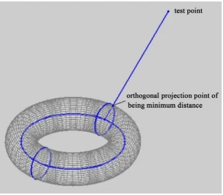
Figure 2. In the case of the test point being not on the center axis of the torus, the corres-ponding orthogonal projection point of being minimum distance.

Remark 1. If the test point

(

x y z0, 0, 0

)

degenerates into the the special point

0

0 0 0 0

1

, 0,

R

x r

x

x z r

R

x _x _R _z _x _R _z

   

−

 _ _ 

 ₊   

 

− + − +

 

 

. In the same way, if the test point

(

x y z0, 0, 0

)

degenerates into

)

0 0

2 ₂ 2 ₂

0

0 0 0 0

1

0, ,

R

y r

y

y z r

R

y _y _R _z _y _R _z

   

−

 _ _ 

 ₊   

 

− + − +

 

 

. Of course, if

the test point

(

x y z0, 0, 0

)

)

is in the inside of the torus, namely,

(

)

2

2 2 2 2

0 0 0

x +y −R +z <r . Firstly, we deal with the first case which the test point is not on the major circle. In fact, analogous to treatment method of the second part content of the second section, it is easy to verify that orthogonal projection point of the test point

(

x y z0, 0, 0

)

is

(

x w y w z w0 0, 0 0, 0 1

)

, where

(

)

0 ₂ ₂ ₂ ₂ ₂

2 2 2

0 0 0 0

0 0 0

1

R R r

w

x y x y

x y R z

 

 

= + −

 

(7)

and

(

)

1 ₂

2 2 2

0 0 0

.

r w

x y R z

=

+ − +

Now we consider the second case which the test point is in the inside of the

torus and is on the major planar circle such that

2 2 2

0 0

0

,

0.

x y R

z

 + =



 ₌

 Similar to the treatment method of the first part

content of second section, it is easy to know that orthogonal projection point set of the test point

(

x y0, 0, 0

)

is

the corresponding minor planer circle. We directly present the corresponding analytical expression according to the test points being at different positions for major planar circle. Since Formula (9) denotes two minor planer circles, in fact, orthogonal projection point set of arbitrary test point being on the major planar circle just only has one minor planar circle. According to this reason, we try to present a unified and concise analytical expression of the only one minor planar circle for arbitrary test point being on the major planar circle. If

0 0, 0 0

x ≠ y ≠ , then the corresponding orthogonal projection point set of the test point

(

x y0, 0, 0

)

is minor

planer circle

( )

0

cos 1 ,

cos 1 , 0 2π

sin .

r

x x

R r

y y

R

z r

θ

θ θ

θ

 ₌  ₊ 

 

 _ _



 ₌  ₊  _{≤ ≤}

 _ _

  =  

(12)

For more special cases, if test point

(

x y z0, 0, 0

)

=

(

R, 0, 0

)

, then orthogonal projection point set of the test

point

(

R, 0, 0

)

is the corresponding minor planer circle

( )

cos ,

0, 0 2π

sin .

x r R

y

z r

θ

θ θ

= +



 = ≤ ≤

  = 

(13)

If test point

(

x y z0, 0, 0

)

= −

(

R, 0, 0

)

, then the corresponding orthogonal projection point set of the test point

(

−R, 0, 0

)

is minor planer circle

( )

cos ,

0, 0 2π

sin .

x r R

y

z r

θ

θ θ

= − −



 = ≤ ≤

  = 

(14)

If test point

(

x y z0, 0, 0

)

=

(

0, , 0R

)

(

0, , 0R

)

( )

0,

cos , 0 2π sin .

x

y r R

z r

θ θ

θ = 

 = + ≤ ≤

  = 

(15)

If test point

(

x y z0, 0, 0

)

=

(

0,−R, 0

)

(

0,−R, 0

)

( )

0,

cos , 0 2π

sin .

x

y r R

z r

θ θ

θ = 

 = − − ≤ ≤

  = 

(8)

Remark 2. In this subsection, we fully present the corresponding orthogonal projection point or point set of arbitrary test point which is in the inside of the torus, namely, the corresponding analytical expression of orthogonal projection point for the minimum distance between the test point and the torus. If the test point is not on the major planar circle, then the corresponding analytical expression of orthogonal projection point is only one point. If the test point is on the major planar circle, then the corresponding analytical expression of orthogonal projection point is minor planar circle. Besides that, if the test point

(

x y z0, 0, 0

)

satisfies the

relationship

(

)

2

2 2 2 2

0 0 0

x +y −R +z =r , it is obviously easy to know that the test point is on the torus.

3. Conclusion

This paper investigates the problem related to a point projection on the torus surface. We present the analytical expression for the orthogonal projection of computing the minimum distance between a point and a torus for all kind s of positions. An area for future research is to develop a method for computing the minimum distance between a point and a general completely center symmetrical surface.

Acknowledgements

We would like to take the opportunity to thank the reviewers for their thoughtful and meaningful comments. This work is supported by the National Natural Science Foundation of China (Grant No. 61263034), the Scientific and Technology Foundation Funded Project of Guizhou Province (Grant No. [2014]2093), the National Bureau of Statistics Foundation Funded Project (Grant No. 2014LY011), the Key Laboratory of Pattern Recognition and Intelligent System of Construction Project of Guizhou Province (Grant No. [2009]4002) and the Information Processing and Pattern Recognition for Graduate Education Innovation Base of Guizhou Province. Linke Hou is supported by the Visiting Scholar Program of the Chinese Scholarship Council (Grant No. 201406225058).

References

[1] Ma, Y.L. and Hewitt, W.T. (2003) Point Inversion and Projection for NURBS Curve and Surface: Control Polygon Approach. Computer Aided Geometric Design, 20, 79-99. http://dx.doi.org/10.1016/S0167-8396(03)00021-9

[2] Yang, H.P., Wang, W.P. and Sun, J.G. (2004) Control Point Adjustment for B-Spline Curve Approximation. Computer- Aided Design, 36, 639-652. http://dx.doi.org/10.1016/S0010-4485(03)00140-4

[3] Johnson, D.E. and Cohen, E. (1998) A Framework for Efficient Minimum Distance Computations. Proceedings of IEEE International Conference on Robotics & Automation, Leuven, 16-20 May 1998, 3678-3684.

http://dx.doi.org/10.1109/robot.1998.681403

[4] Piegl, L. and Tiller, W. (2001) Parametrization for Surface Fitting in Reverse Engineering. Computer-Aided Design, 33, 593-603. http://dx.doi.org/10.1016/S0010-4485(00)00103-2

[5] Pegna, J. and Wolter, F.E. (1996) Surface Curve Design by Orthogonal Projection of Space Curves onto Free-Form Surfaces. Journal of Mechanical Design, 118, 45-52. http://dx.doi.org/10.1115/1.2826855

[6] Besl, P.J. and McKay, N.D. (1992) A Method for Registration of 3-D Shapes. IEEE Transactions on Pattern Analysis and Machine Intelligence, 14, 239-256. http://dx.doi.org/10.1109/34.121791

[7] Mortenson, M.E. (1985) Geometric Modeling. Wiley, New York.

[8] Zhou, J.M., Sherbrooke, E.C. and Patrikalakis, N. (1993) Computation of Stationary Points of Distance Functions. En-gineering with Computers, 9, 231-246. http://dx.doi.org/10.1007/BF01201903

[9] Johnson, D.E. and Cohen, E. (2005) Distance Extrema for Spline Models Using Tangent Cones. Proceedings of the

2005 Conference on Graphics Interface, Victoria, May 9-11, 2005, 3 p.

[10] Hartmann, E. (1999) On the Curvature of Curves and Surfaces Defined by Normalforms. Computer Aided Geometric Design, 16, 355-376. http://dx.doi.org/10.1016/S0167-8396(99)00003-5

[11] Limaien, A. and Trochu, F. (1995) Geometric Algorithms for the Intersection of Curves and Surfaces. Computers & Graphics, 19, 391-403. http://dx.doi.org/10.1016/0097-8493(95)00009-2

(9)

[13] Press, W.H., Teukolsky, S.A., Vetterling, W.T. and Flannery, B.P. (1992) Numerical Recipes in C: The Art of Scien-tific Computing. 2nd Edition, Cambridge University Press, New York.

[14] Elber, G. and Kim, M.S. (2001) Geometric Constraint Solver Using Multivariate Rational Spline Functions. Proceed-ings of the Sixth ACM Symposium on Solid Modeling and Applications, 1-10. http://dx.doi.org/10.1145/376957.376958 [15] Patrikalakis, N. and Maekawa, T. (2001) Shape Interrogation for Computer Aided Design and Manufacturing. Springer

Verlag.

[16] Chen, X.D., Xu, G., Yong, J.H., Wang, G.Z. and Paul, J.C. (2009) Computing the Minimum Distance between a Point and a Clamped B-Spline Surface. Graphical Models, 71, 107-112. http://dx.doi.org/10.1016/j.gmod.2009.01.001 [17] Selimovic, I. (2006) Improved Algorithms for the Projection of Points on NURBS Curves and Surfaces. Computer

Aided Geometric Design, 23, 439-445. http://dx.doi.org/10.1016/j.cagd.2006.01.007

[18] Cohen, E., Lyche, T. and Riesebfeld, R. (1980) Discrete B-Splines and Subdivision Techniques in Computer-Aided Geometric Design and Computer Graphics. Computer Graphics and Image Processing, 14, 87-111.

http://dx.doi.org/10.1016/0146-664X(80)90040-4

[19] Piegl, L. and Tiller, W. (1995) The NURBS Book. Springer, New York. http://dx.doi.org/10.1007/978-3-642-97385-7

[20] Chen, X.D., Yong, J.H., Wang, G.Z., Paul, J.C. and Xu, G. (2008) Computing the Minimum Distance between a Point and a NURBS Curve. Computer-Aided Design, 40, 1051-1054. http://dx.doi.org/10.1016/j.cad.2008.06.008

[21] Liu, X.-M., Yang, L., Yong, J.-H., Guf, H.-J. and Sun, J.-G. (2009) A Torus Patch Approximation Approach for Point Projection on Surfaces. Computer Aided Geometric Design, 26, 593-598. http://dx.doi.org/10.1016/j.cagd.2009.01.004 [22] Hu, S.M. and Wallner, J. (2005) A Second Order Algorithm for Orthogonal Projection onto Curves and Surfaces.

Computer Aided Geometric Design, 22, 251-260. http://dx.doi.org/10.1016/j.cagd.2004.12.001