Munich Personal RePEc Archive
Health care expenditure and GDP: An
international panel smooth transition
approach
Chakroun, Mohamed
University of Sfax, Faculty of Business and Economics
May 2009
Online at
https://mpra.ub.uni-muenchen.de/17493/
Health care expenditure and GDP:
An international panel smooth transition approach
Mohamed Chakroun1#
URED, Université de Sfax, Tunisia
Abstract
In this paper, we investigate the potential threshold effects in the relationship between
national expenditures on health care and national income. Using a panel threshold regression
model, we derive country-specific and time-specific income elasticities for 17 OECD
countries over the period 1975–2003. In contrast to many previous analyses, our empirical
results show that health care is a necessity rather than a luxury. Further, the relationship
between health expenditure and income seems rather nonlinear, changing over time and
across countries.
JEL classification: C12
Keywords: Health expenditure; Income elasticity; Panel smooth threshold regression models
1. Introduction
It is well known that a significant relationship exists between national expenditures on health
care and national income. Thirty years ago, Joseph Newhouse (1977) observed on the basis of
an analysis of a cross-section of thirteen developed countries that over 90 percent of the
variation between countries in per capita medical care expenditure could be explained by
variations in per capita GDP. In an Engel curve context, this means that health care is a
‘‘luxury’’ good. Afterwards, growing attention has been paid for the determinants of
aggregate health care expenditure (Parkin et al., 1987; Gerdtham et al., 1992; Hitris and
1
Corresponding author. Faculté des sciences économiques et de Gestion de Sfax, URED. Route de l’aérodrome km 4,5-BP 1088- 3018 Sfax, Tunisie. Tel. : + 216 21 059 589 (+ 216 98 488 559); fax: + 216 74 279 139; e-mail addresses : chakroun_mohamed2000@yahoo.fr;
Posnett, 1992; Hansen and King, 1996; Blomqvist and Carter, 1997; Di Matteo and Di
Matteo, 1998; Okunade and Karakus, 2001; Clemente et al., 2004; Dregers and Reimers,
2005; OECD, 2006; Tosetti and Moscone, 2007; Hartwig, 2008; etc.). Most estimates of the
income elasticity of health care spending obtained, especially those derived from aggregative
cross-section or time series data, exceed unity. But, as pointed by Blomqvist and Carter
(1997) “the idea that health care spending should behave as a luxury good when aggregate
data are used appears puzzling”. In the same way, Clemente and al. (2004) argued that this
finding seems counter-intuitive from an economic point of view.
Two potential reasons can be advanced to explain why the demand for health care may
mistakenly have an income elasticity in excess of unity. The first one is the potential
non-stationarity of the data. As explained by Jewel et al. (2003), when examining the relationship
between health expenditures (HE) and GDP it is important to determine whether or not these
two variables are stationary. Empirical tests that ignore this issue can lead to spurious
regressions and meaningless results. Recently, many studies, using both country-by-country
and panel data techniques, have attempted to analyze the time series pattern of these two
variables. (Mc-Coskey and Selden, 1998; Roberts, 1999; Gerdtham and Lothgren, 2000;
Okunade and Karakus, 2001; Jewell et al., 2003; Carrion-i-Silvestre, 2005; Dreger and
Reimers, 2005). Most of these found that HE and GDP are non-stationary (for example,
Hansen and King, 1996; Blomqvist and Carter, 1997; Roberts (1999); Gerdtham and
Lothgren, 2000). The second reason, which is specific to the panel data models, concerns
cross-section heterogeneity. Pesaran and Smith (1995) and Hsiao (2003) have already
indicated that ignorance of this issue causes biases to appear. Thus, in presence of
heterogeneity, assuming a common elasticity of output with respect to health expenditure
cross-country data are characterised by strong heterogeneity that, if not properly incorporated in
econometric models, could lead to the estimation of an income elasticity greater than one.
One solution to deal with this heterogeneity problem is to specify a Panel Smooth Threshold
Regression (PSTR) model, recently developed by Fok et al. (2004), González et al. (2005),
Colletaz and Hurlin (2005) and Fouquau et al. (2008), which allows for smooth changes in
country-specific correlations and cross-country heterogeneity and time instability of the
elasticity. Such an approach is then suitable to capture both cross-country heterogeneity and
time variability of the GDP-HE correlations2.
The remainder of the paper is organised as follows. In section 2, we discuss the threshold
specification of the determinants of health care expenditure. The choice of the threshold
variable, linearity tests and estimates for the parameters are presented in section 3. The data
and the results are presented in section 4, while the final section concludes.
2. A PSTR model of health care expenditure
Our ambition in this paper is to test whether or not health care expenditure is a luxury good.
To address this question, we consider the following model:
heit =αi +β.capitait +εit, i =1,...,N, t =1,...,T (1)
where and denotes, respectively, the logarithm of real per-capita health
expenditure and the logarithm of real per-capita income in the i
it
he capitait
th
country at time t, both
expressed in purchasing power parity (PPP). αi is an individual fixed effect, and εit is the
error term. As argued by Hitris and Posnett (1992), the use of health specific PPP to convert
health spending provides a comparison of the real quantity of health care services purchased
with given expenditure.
2
Nevertheless, this model suffers from two major problems. Firstly, many other factors, in
addition to income, could affect health care expenditure. The share of the elderly, medical
progress and relative prices are often mentioned to be the main non-income factors underlying
health expenditure growth in the OECD countries. Many studies have previously found a
positive and significant relationship between health care spending and the proportion of
population over 65 (see for example Kleiman, 1974; Leu, 1986; Hitiris and Posnett, 1992,
Felder et al., 2000). As highlighted by Hansen and King (1996), the elderly consume more
health per capita than people of working age. Recently, the OECD (2006) points out that
across all health expenditures types, expenditure on those aged over 65 is around four times
higher than on those under 65. Further, between 1981 and 2002, average growth of public
health spending was by 3.6% per year for OECD countries, of which 0.3% point was directly
linked to demographic effects. On the other hand, Leu (1986) and Kleiman (1974) found a
significant relationship between health expenditure and the proportion of population under 15.
Kleiman (1974) reports a negative correlation between these two variables. He explained his
result by the low per unit cost of the goods and services young people consume, such as
vaccinations.
Whatever the relationship between the population structure and health spending may be,
population ageing is a common fact in developed countries. Progress in medical technology
and treatment is advanced to be one of the most important determinants of health outcomes
during the last century. As suggested by Blomqvist and Carter (1997) and later by Tosetti and
Moscone (2007), the rising of health care expenditure has been to a large extent driven by
changes in technology and treatment. Newhouse (1992) and Wanless (2001) have already
explained that technical progress causes a decrease of the relative price of health goods and
services. If so, the more elastic is the demand for health care, the more increasing will be
Another determinant of health care expenditure that has been identified by the literature is the
share of public financing. In OECD countries, health care is mainly financed through public
funds. Leu (1986) argued that the share of public financing increases health care expenditure
to the extent that it reduces the price to the consumer. However, his argument is not
confirmed by recent empirical studies. Gerdtham et al. (1992) and recently Tosetti and
Moscone (2007) have found a negative relationship between the proportion of health care
expenditure that is publicly funded and total health expenditure.
Thus, given the potential interrelations between health care expenditure and these non-income
factors, they should be included in the regression model as additional explanatory variables to
check the robustness of the estimated income elasticity. But even in doing so, the problem is
not resolved since the conditional relationship between income and health spending is always
assumed homogeneous. In fact, equation (1) assumes the same income elasticity across the N
countries of the panel, i.e.βi =β,∀i=1,...,N. Such an assumption is somewhat restrictive
since there is substantial differences among OECD countries in the financing and organization
of health services production, which may causes differences in the aggregate demand
functions of health services (Clemente et al., 2004).
Besides, equation (1) implies that the income elasticity is constant for the set time period of
the model. This assumption seems to be misleading especially when dealing with large time
dimension panels. Clemente and al. (2004) believe that it is too restrictive to assume an
unchangeable relationship between health spending and the GDP for OECD countries.
Usually, it is difficult to resolve heterogeneity and time variability problems simultaneously.
But one issue proposed in the literature consists in introducing threshold effects in a linear
panel model specification. Let us consider a Panel Smooth Threshold Regression (PSTR)
change smoothly as a function of a threshold variable. In the case of two extreme regimes and
one transition function, the model can be presented by3 :
heit =αi +β0.capitait +β1.capitait.g(qit;γ,c)+εit (2)
The transition function is then given by :
, 0 )] .( exp[ 1 1 ) , ; ( > − − + = γ γ γ c q c q g it
it (3)
Thus, the income elasticity is defined as a weighted average of parameters β0and β1. For a
given threshold variable, the elasticity of health care spending with respect to income for the
ith country at time t is equal to:
0 1.g(q ; ,c)
capita he
eity =β +β it γ
∂ ∂
= , with (4)
⎪⎩ ⎪ ⎨ ⎧ < ≤ ≤ + > + ≤ ≤ 0 if 0 if 1 0 1 0 1 1 0 0 β β β β β β β β y it y it e e
Note that parameters β0 and β1 do not correspond to income elasticity. A positive (negative)
value of β1 simply indicates an increase (decrease) of the elasticity with the value of the
threshold variable.
3. Estimation and specification tests
In a threshold model, there are two main problems of specification: the choice of the threshold
variable and the determination of the number of regimes. Following Colletaz and Hurlin
(2006) and Fouquau et al. (2008), we adopt a three-step procedure for estimating the final
PSTR model. First, we test the linearity against the PSTR model. Then, if linearity is rejected,
we determine the number of transition functions. Finally, we remove individual-specific
means and then we apply non linear least squares to estimate the parameters of the
transformed model.
3
Note that the PSTR model can be generalised to r + 1 extreme regimes as follows:
it j j it j it r j j it i
it capita capita g q c
he =α +β +
∑
β γ +ε3.1 Choice of the threshold variable
What determines the size of the income elasticity? There are at least two factors which could
affect the shape of the income/expenditure relationship: price variation and technological
progress.
As advanced by Baumol (1967), health sector is highly labor-intensive. Besides, it produces
commodities for which the price elasticity is very low. Then, relying on this assumption, the
relative price of these commodities tends to rise with income (Blomqvist and Carter,1997)
and so does health expenditure. Clemente et al. (2004) consider that “with the price of health
care growing faster than the average, health expenditure grows at a faster rate than income”.
Nevertheless, as pointed out by Hartwig (2008), medical care price indices should not be used
as explanatory variables, especially in cross-country studies, because, he reported, “price
trends in health care must be expected to be as diverse as national schemes of price
regulation”. Besides, Newhouse (1977) argued that price cannot be considered as a relevant
determinant of health care spending in west countries because non-market rationing
dominates.
Another factor being thought to play a major role in determining the shape of the
income/expenditure relationship is medical progress. Baumol (1993) believes that health care
is “an industry whose costs are driven by technological imperatives to rapid rise”. Feldstein
(1995) argues that “the rising cost of hospital care has been driven by changes in the
technology or style or quality of care”. Although someone should expect technical progress to
be cost-saving, in the sense that it reduces the relative price of health facilities and permits,
consequently, a decrease in health expenditure4, it appears that such a proposal is to some
extent unreliable. Many studies suggest that technical change has a strong cost-increasing
effect in health care (see for example, Weisbrod, 1991; Blomqvist and Carter, 1997; Clemente
4
et al., 2004). Blomqvist and Carter (1997) explained that what is really purchased by
individuals is ‘good health’, not health services. Then, “technical change takes the form of
progress in our ability to transform health services into ‘good health’, rather than reducing the
resource cost of producing health services”. The same idea has been developed by Clemente
et al. (2004). They argue that individuals are increasingly interested in the quality of their life
more than in the quantity of health care they consume. This explains why individuals devote
an increasing fraction of their income to health services. The candidate for the threshold
variable considered in this study is technical progress. Following Dreger and Reimers (2005),
life expectancy is employed as a proxy, since data on medical technologies are incomplete.
3.2. Linearity tests
As explained by Fouquau et al. (2008), to test linearity in the PSTR model (equation 2) we
replace the transition function g(qit;γ,c)by its first-order Taylor expansion around γ =0.
We then obtain an auxiliary regression:
heit =αi +θ0.capitait +θ1.capitait.qit +εit (5)
Thus, the linearity test consists of testingH0:θ1 =0. If linearity is rejected, a sequential
approach is used to test the null hypothesis of no remaining nonlinearity in the transition
function5. If we denote the panel sum of squared residuals under (linear panel model
with individual effects) and the panel sum of squared residuals under (PSTR model
with two regimes), the corresponding F-statistic is then given by:
0
SSR H0
1
SSR H1
[
(
)
]
(
[
SSR TN N K)
]
K SSR SSRLMF
− − − =
/
/
0
1
0 (6)
5
Testing for non remaining nonlinearity consists of checking whether there is one transition function (H0:r=1 ) or whether there are at least two transition functions (H1:r=2). For more details, see Fouquau et
where K is the number of explanatory variables . Under the null hypothesis, the LM statistic is
distributed as a and the F-statistic has an approximate
distribution. ) ( 2 K χ
[
K TN N r K]
F , − −( +1)
4. Data and results
The data set consists of a pooled sample of time-series and cross-section observations
covering 176 OECD countries for the 29 years 1975-2003: a total of 493 observations. Some
countries were excluded from the study because it was not possible to obtain detailed health
care expenditure statistics starting from 1975. Our data are taken from OECD Health
Database (2007) and World Development Indicators (WDI, 2005).
In this study, we propose to estimate a multivariate regression model. Real per capita health
expenditure (he) is modelled conditioned on real income per capita (capita), the share of the
elderly (POP65), the proportion of population under 15 (POP15) and the share of public
financing (PUB). The threshold variable chosen is life expectancy, as a proxy for technical
progress. We begin the analysis by estimating the basic model proposed by Newhouse (model
1). Then, we introduce new variables reflecting changes in population structure and
institutional arrangements (model 2 and model 3).
The econometric framework of our analysis is the following:
(7) c q g capita capita he : 1
Model it =αi +β0. it +β1. it. ( it;γ, )+εit
[
capita POP]
g(
q C)
(8) POP capita he 2 Model it j j it j r j it j it j it it i it ε γ η β η β α + + + + + =∑
= , ; . 65 . . 65 . . : 1 0 0[
capita PUB POP]
g(
q C)
(9) POP PUB capita he 3 Model it j j it j r j it j it j it j it it it i it ε γ λ ξ β λ ξ β α + + + + + + + =∑
= , ; . 15 . . . 15 . . . : 1 0 0 0 6The first step is to test the log-linear specification of the three models. The results of these
linearity tests and specification tests of no remaining nonlinearity are reported on Table 1. As
explained by Fouquau et al. (2008), the threshold variable may have a direct effect on the
dependant variable. In this case, one could misleadingly find switching. To check this point
we conduct a second test of non remaining linearity with direct effects in which the threshold
variable is used as an explanatory variable.
Table 1. Tests of linearity
LMF test for remaining linearity
Specification Model 1 Model 2 Model 3
Explicative variables Real capita Real capita, POP 65 Real capita, PUB, POP 15
1 : vs. 0
: 1
0 r= H r=
H 131,153(0,00) 31,142(0,00) 65,058(0,00)
2 : vs. 1
: 1
0 r= H r=
H 0,231(0,631) 1,181(0,308) 0,171(0,916)
3 : vs. 2
: 1
0 r= H r=
H - - -
LMF test for remaining linearity with direct effects
Specification Model 1 Model 2 Model 3
Explicative variables Real capita Real capita, POP 65 Real capita, PUB, POP 15
1 : vs. 0
: 1
0 r= H r=
H 8,493(0,00) 12,833(0,00) 25,523(0,00)
Notes: The threshold variable is life expectancy. The corresponding LMF statistic has an asymptoticF
[
K,TN−N−(r+1)K]
distribution underH0, where K is the number of explicative variables. The corresponding p-values are reported in parentheses.
The linearity tests clearly lead to the rejection of the null hypothesis of linearity for all three
models, whether direct effects are considered or not. The strongest rejection of the null of
linearity is obtained when model 1 is considered. This result implies that there is strong
evidence that the relationship between health expenditure and income is non-linear. Thus,
using a linear panel model in which income elasticity is assumed homogenous across
countries may possibly lead to fallacious estimates, since the estimated elasticity could vary
income/health expenditure relationship changes with time, in response to potential structural
changes in financing schemes, health policies, economic conditions, etc. In this case, a linear
approach which offers an average estimate of the different historical values of the income
elasticity could hide information about the above structural changes.
Table 1 gives also information about the optimal number of transition functions. The
specification tests of no remaining nonlinearity lead to the identification of two extreme
[image:12.595.70.527.279.642.2]regimes (r = 1).
Table 2. Parameters estimates for the final PSTR models
Specification Model 1 Model 2 Model 3
Explicative variables Real capita Real capita, POP 65 Real capita, PUB,
POP 15
r* 1 1 1
__________________________________________________________________________________________
Parameter
β
0 0,82(0,08) 0,8374(0,06) -4,7712(0,54)Parameter
β
1 0,0961(0,01) 0,0458(0,03) 6,3131(0,59)Parameter
η
0 - 0,3943(0,08) -Parameter
η
1 - -0,0334(0,12) -Parameter ξ0 - - 11,3795(1,12)
Parameter ξ1 - - -13,2138(1,31)
Parameter
λ
0 - - -0,4703(0,98)Parameter
λ
1 - - 0,1384(1,08)_________________________________________________________________________________________ Location parameters C 4,3517 4,3354 4,0317
Slopes parameters
γ
23,5477 52,8099 6,6653Notes: The threshold variable is life expectancy. The standard errors for coefficients in parentheses are corrected for heteroskedasticity. The PSTR parameters can not be directly interpreted as elasticities.
Table 2 reports the parameter estimates of the final PSTR models. As explained in section 2,
the estimated parameters cannot be directly interpreted as elasticities. Let us consider the
increases, income elasticity increases. In other words, with population being ageing,
preference of households for health increases. Becoming more interested in the quality of
their life, they will spend an increasing amount of revenue (savings) to purchase advanced
health facilities.
Model 1 Model 2 Model 3
y
e σ ey σ epop65 σ ey σ epub σ epop15 σ
Germany 0,853 (0,01) 0,854 (0,01) 0,382 (0,01) 0,730 (0,13) -0,136 (0,27) -0,350 (0,00) Australia 0,862 (0,01) 0,862 (0,01) 0,376 (0,01) 0,811 (0,12) -0,305 (0,26) -0,348 (0,00) Austria 0,852 (0,01) 0,854 (0,01) 0,382 (0,01) 0,717 (0,15) -0,108 (0,31) -0,350 (0,00) Canada 0,864 (0,01) 0,865 (0,01) 0,374 (0,01) 0,838 (0,10) -0,361 (0,21) -0,347 (0,00) Denmark 0,851 (0,01) 0,852 (0,01) 0,384 (0,01) 0,731 (0,06) -0,137 (0,13) -0,350 (0,00) Spain 0,863 (0,01) 0,863 (0,01) 0,375 (0,01) 0,825 (0,10) -0,334 (0,20) -0,348 (0,00) USA 0,851 (0,01) 0,852 (0,01) 0,384 (0,01) 0,726 (0,08) -0,126 (0,18) -0,350 (0,00) Finland 0,852 (0,01) 0,853 (0,01) 0,383 (0,01) 0,724 (0,12) -0,121 (0,25) -0,350 (0,00) Iceland 0,871 (0,01) 0,871 (0,01) 0,370 (0,01) 0,892 (0,07) -0,474 (0,15) -0,346 (0,00) Japan 0,874 (0,01) 0,871 (0,01) 0,370 (0,01) 0,907 (0,11) -0,506 (0,22) -0,346 (0,00) Norway 0,863 (0,01) 0,863 (0,01) 0,375 (0,01) 0,829 (0,07) -0,342 (0,14) -0,348 (0,00)
New-Zealand 0,853 (0,01) 0,855 (0,01) 0,382 (0,01) 0,735 (0,13) -0,146 (0,28) -0,350 (0,00) Netherlands 0,862 (0,01) 0,863 (0,01) 0,376 (0,01) 0,823 (0,06) -0,329 (0,13) -0,348 (0,00) UK 0,854 (0,01) 0,855 (0,01) 0,381 (0,01) 0,745 (0,11) -0,167 (0,23) -0,349 (0,00) Sweden 0,867 (0,01) 0,867 (0,01) 0,373 (0,01) 0,863 (0,08) -0,414 (0,17) -0,347 (0,00) Ireland 0,848 (0,01) 0,850 (0,01) 0,385 (0,01) 0,686 (0,12) -0,042 (0,26) -0,351 (0,00) Portugal 0,845 (0,01) 0,849 (0,01) 0,386 (0,01) 0,642 (0,17) 0,050 (0,35) -0,352 (0,00)
[image:13.595.72.533.214.481.2]All countries 0,858 (0,01) 0,859 (0,01) 0,379 (0,01) 0,778 (0,13) -0,235 (0,27) -0,349 (0,00) Table 3. Income elasticities of health care spending: average of individual PSTR estimates.
Notes: For each country, the average, e, and standard deviation, σ ,of the estimated elasticities are reported. The threshold variable is life expectancy.
Given the parameters estimates of the final PSTR models, it is now possible to compute, for
each country of the sample and for each date, the time varying elasticities of health care
spending with respect to income ( ), the share of the elderly ( ), the proportion of
population under 15 ( ) and public spending ( ). These smoothed individual
elasticities are given by the formula (4). The average estimated elasticities are reported in
Table 3 for the three PSTR models. These estimated elasticities are based on the historical
values of the transition variable, life expectancy, observed for the 17 OECD countries.
y it
e eitpop65
15
pop it
As can be seen, the income elasticity of health care spending is below unity for all the
countries of the sample whatever the model considered. This result contrasts with that found
in previous studies: here, health care is not a luxury good. Some remarks can be driven from
table 3. When considering models 1 and 2, the income elasticity does not considerably change
from one country to another. But, when public spending is introduced as an explanatory
variable (model 3), our results slightly change. Except for Iceland and Japan, the income
elasticity is being lower. Tosettiy and Moscone (2007) found the same result arguing that
introduction of public spending in the regression weakens the link between income and the
standard of care. Another interesting finding is that coefficients are being different from one
country to another, ranging from 0,642 in Portugal to 0,907 in Japan. This result obviously
shows the heterogeneity of the income elasticity among OECD countries.
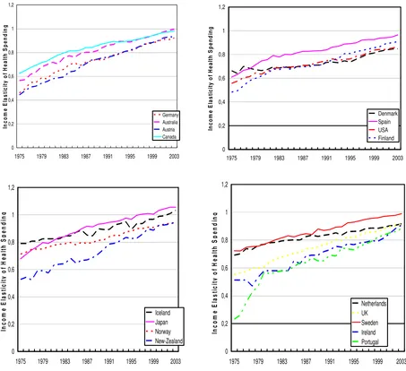
Exhibiting cross-country heterogeneity is not the only advantage of a PSTR model. Such a
specification permits in addition to study the time variability of the estimated income
elasticities of health care spending. On the figure (1), the estimated elasticities of health
expenditure with respect to real income are plotted over the period 1975-2003 for the 17
countries of our sample.
y it
e
Plots have been done only for model 3 in order to capture as large as possible cross-country
heterogeneity. Besides, we can observe from table 2 that for model 3 the estimated slope
parameter γ is relatively small. This implies that the transition between extreme regimes is
smooth. But whatever the model considered, the finding is always the same: for all the
0 0,2 0,4 0,6 0,8 1 1,2
1975 1979 1983 1987 1991 1995 1999 2003
In co m e E las ti ci ty o f H e a lt h S p en d in g Germany Australia Austria Canada 0 0,2 0,4 0,6 0,8 1 1,2
1975 1979 1983 1987 1991 1995 1999 2003
In com e E last ic it y of H e a lt h S p end in g Denmark Spain USA Finland 0 0,2 0,4 0,6 0,8 1 1,2
1975 1979 1983 1987 1991 1995 1999 2003
In co m e E last ici ty o f H eal th S p en d in g Iceland Japan Norway New-Zealand 0 0,2 0,4 0,6 0,8 1 1,2
1975 1979 1983 1987 1991 1995 1999 2003
[image:15.595.56.509.76.490.2]In c o m e E las ti ci ty of H e a lt h S p en d in g Netherlands UK Sweden Ireland Portugal
Figure 1 : Estimated individual income elasticities
Such a result sustains the proposal of a shift towards a growing and strongest relationship
between health care spending and income in OECD countries. For nine countries of the
sample (Germany, Austria, Spain, Finland, Norway, New-Zealand, Netherlands,
United-kingdom and Ireland), income elasticity is superior to 0,9 at the end of the period. For three
countries (Australia, Canada and Sweden), this elasticity is around unity. For Japan and
Iceland, it exceeds unity. What these results tell us? Is health care really becoming a luxury
good? Recall that these estimated elasticities are based on the historical values of the
transition variable, life expectancy, observed for the 17 OECD countries. So, one plausible
given threshold, the individual’s preferences shift towards health at the expense of
consumption goods, and additional resources are required to enjoy a longer life. As
technology of life extension is subject to “sharp diminishing returns” (Hall and Jones, 2005),
a more than proportionate part of income will be needed in order to extend life. Accordingly,
the more the people get richer, the more the share of resources they are willing to devote to
health care increases. Of course, life expectancy is used in our PSTR model as a proxy for
medical progress. Many previous studies have already pointed out that technical change is the
main factor underlying health expenditure growth in the OECD countries. In our opinion, this
purpose particularly matters in societies whose age pyramid dramatically switches in favour
of the elderly. To examine this, we have re-estimated our PSTR model by taking the share of
the elderly as a threshold variable. Not surprisingly, we found an income elasticity well above
unity7. From this point of view, the idea that health care is a luxury good, and that at the
margin health care may contribute more to ‘caring’ than to ‘curing’ holds good.
5. Conclusions
Heterogeneity and nonlinearity can lead to biased results when trying to model the
relationship between income and health care expenditure. If these two topics are not well
incorporated in econometric models, it is likely that estimates misleadingly reveal an income
elasticity greater than unity. Generally, it is difficult to resolve heterogeneity and nonlinearity
problems simultaneously. But one issue proposed in the literature consists in introducing
threshold effects in a linear panel model specification. Smooth transition regression models
are straightforward to deal with cross-country heterogeneity and time instability of the
elasticities by allowing coefficients to vary across individuals and over time.
In this paper we used a panel smooth transition regression model to estimate the relationship
between income and health care expenditure for 17 OECD countries over the period
1975-2003. In contrast to many previous studies, we show that, on average, the income elasticity of
health care spending is below unity for all the countries considered in the study. This finding
is robust to the inclusion of other non-income determinants of health expenditure in the
regression. But, in all likelihood, it seems that the shape of the income/expenditure
relationship is changing over time, especially when introducing public health expenditure as
an additional explanatory variable. Our estimates show that the income elasticity of health
care spending is constantly increasing between 1975 and 2003. For fourteen countries, this
elasticity grows to be close to unity at the end of the period. Questioning why the income
elasticity increases over time, we have advanced the idea that when life expectancy exceeds a
given threshold, the medical care needed by older people to enjoy longer life involves
expansive technology and hospitalization. But, at this particular stage, health is directly
affecting welfare and people are willing to purchase those expansive health care facilities as
much as they afford it. As the population get richer and older, the share of health expenditure
in the total resources raises and the income elasticity is increasingly high that the proportion
of the elderly increases.
Finally, the main results of the paper can be summarized as follow: (i) the relationship
between income and health care expenditure is nonlinear, (ii) on average the income elasticity
of health care spending is below unity for the 17 OECD countries of the sample, (iii) the
relationship between income and health spending is changing over time and across countries
and, (iv) health expenditure seems to behave as a luxury good when life expectancy exceeds a
critical threshold.
References
Baumol, W.J. (1967) Macroeconomics of unbalanced growth: the anatomy of urban crisis.
Baumol, W.J. (1993) Health care, education and the cost disease: a looming crisis for public
choice. Public Choice 77 (1), 17–28.
Blomqvist, A.G., Carter, R.A.L. (1997) Is health care really a luxury? Journal of Health
Economics 16 (2), 207–229.
Carrion-i-Silvestre, J.L. (2005) Health care expenditure and GDP: are they broken stationary?
Journal of Health Economics 24 (5), 839–854.
Clemente, J., Marcuello, C., Montañés, A., Pueyo, F. (2004) On the international stability of
health care expenditure functions: are government and private functions similar? Journal of
Health Economics 23, 589–613.
Colletaz, G., Hurlin, C. (2006) Threshold effects in the public capital productivity: an
international panel smooth transition approach. University of Orléans. Working paper.
Di Matteo, L., Di Matteo, R. (1998) Evidence on the determinants of Canadian provincial
health expenditures 1965–1991. Journal of Health Economics 17 (2), 211–228.
Dreger, C., Reimers, H.E . (2005) Health care expenditures in OECD countries: a panel unit
root and cointegration analysis. International Journal of Applied Econometrics and
Quantitative Studies. Vol.2-2.
Felder, S., Meier, M., Schmitt, H. (2000) Health care expenditure in the last months of life.
Journal of Health Economics 19, 679–695.
Feldstein, M. (1995) The economics of health and health care: what have we learned? What
have I learned? AEA Papers and Proceeding 28, 31.
Fok, D., van Dijk, D., Franses, P. (2004) A multi-level panel STAR model for US
manufacturing sectors. Working Paper University of Rotterdam.
Fouquau, J., Hurlin, C., Rabaud, I. (2008) The Feldstein–Horioka puzzle: a panel smooth
Gerdtham, U.-G., Lothgren, M. (2000) On stationarity and cointegration of international
health expenditure and GDP. Journal of Health Economics 19 (4), 461–475.
Gerdtham, U.G., Sogaard, J., Andersson, F., Jonsson, B. (1992) An econometric analysis of
health care expenditure: a cross-section study of the OECD countries, Journal of Health
Economics 11, 63.
González, A., Teräsvirta, T., van Dijk, D. (2005) Panel smooth transition regression model.
Working Paper Series in Economics and Finance, vol. 604.
Hall, R., Jones, C.I. (2005) The value of life and the rise in health spending. Working Paper.
Hansen, B.E. (1999) Threshold effects in non-dynamic panels: estimation, testing and
inference. Journal of Econometrics 93, 345-368.
Hansen, P., King, A. (1996) The determinants of health care expenditure: a cointegration
approach. Journal of Health Economics 15 (1), 127–137.
Hartwig, J. (2008)What drives health care expenditure?—Baumol’s model of ‘unbalanced
growth’ revisited. Journal of Health Economics 27, 603–62
Hitiris, T., Posnett, J. (1992) The determinants and effects of health expenditure in developed
countries. Journal of Health Economics 11 (2), 173–181.
Hsiao, C. (2003) Analysis of panel data, econometric society monographs. Cambridge
University Press.
Jewell, T., Lee, J., Tieslau, M., Strazicich, M.C. (2003) Stationarity of health expenditures
and GDP: evidence from panel unit root tests with heterogeneous structural breaks. Journal of
Health Economics 22 (2), 313–323.
Kleiman, E. (1974) The determinants of national outlays on health. In: Perlman, M. (Ed.), The
Leu, R.E. (1986) The public–private mix and international health care costs. In: Culyer, A.J.,
Jönsson, B. (Eds.), Public and Private Health Care Services: Complementarities and Conflicts.
Basil Blackwell, Oxford.
McCoskey, S.K., Selden, T.M. (1998) Health care expenditures and GDP: panel data unit root
test results. Journal of Health Economics 17 (3), 369–376.
Newhouse, J. (1992) Medical care costs: how much welfare loss? Journal of Economic
Perspectives 6 (3), 3–21.
Newhouse, J.P. (1977) Medical-care expenditure: a cross-national survey. Journal of Human
Resources 12 (1), 115–125.
OECD. (2006) Projecting OECD health and long-term care expenditures: what are the main
drivers? OECD Economics Department Working Papers, No. 477.
Okunade, A.A., Karakus, M.C. (2001) Unit root and cointegration tests: time-series versus
panel estimates for international health expenditure models. Applied Economics 33 (9), 1131–
1137.
Parkin, D., McGuire, A., Yule, B. (1987) Aggregate health care expenditures and national
income: is health care a luxury good? Journal of Health Economics 6 (2), 109–127.
Pesaran, H.M., Smith, R. (1995) Estimating long-run relationships from dynamic
heterogenous panels. Journal of Econometrics 68, 79-113.
Roberts, J., 1999. Sensitivity of elasticity estimates for OECD health care spending: analysis
of a dynamic heterogeneous data field. Health Economics 8 (5), 459–472.
Tosetti, E., Moscone, F. (2007) Health expenditure and income in the United States.
University of Leicester, Working Paper No. 07/14
Wanless, D. (2001) Securing our future health: taking a long-term view. Interim Report, HM
Weisbrod, B. (1991) The health care quadrilemma: an essay on technological change,