Determinants of Exports in Pakistan: An Econometric Analysis (1970 2006)

Munich Personal RePEc Archive

Determinants of Exports in Pakistan: An

Econometric Analysis (1970-2006)

Khattak, Naeem Ur Rehman Khattak and Hussain, Anwar

Hussain

Pakistan Instittute of Development Economics Islamabad Pakistan

2010

Online at

https://mpra.ub.uni-muenchen.de/41988/

DETERMINANTS OF EXPORTS IN PAKISTAN: AN ECONOMETRIC

ANALYSIS (1970-2006)

Naeem-ur-Rehman Khattak* and Anwar Hussain**

ABSTRACT

The present study has been conducted in the year 2008 to assess the determinants of

exports in Pakistan during 1970-2006 using econometric techniques. Time series data

ranging from 1970 to 2006 on total exports, primary commodities exports,

semi-manufactures and exports of manufactured goods has been taken from Economic Survey

of Pakistan (Statistical Supplement, 2006-07). Augmented Dickey Fuller (ADF) test has

been used for checking the stationarity of the data. Furthermore, the Johenson

Co-integration test (likelihood ratio statistic) has been used to detect the long-term

relationship among the series. The method of ordinary least square has been used to

assess the determinants of exports in Pakistan. The results indicate that 1% increase in the

exports of primary commodities brings 0.97% increase in total exports in Pakistan.

Similarly, 1% increase in the exports of semi-manufactures leads to increase total exports

by 0.99%. On similar pattern, 1% increase in the exports of manufactured goods leads to

increase total exports by 1%. The coefficients of all the explanatory variables are

statistically significant at both 5% and 1% level of significance. It is recommended to

increase the exports of primary goods, semi-manufactures and manufactured goods so as

make balance of trade favorable.

Key words: Determinants; exports; econometric; analysis

INTRODUCTION

The exports of Pakistan are based on primary commodities, semi-manufactures and

manufactured goods. These include fish, rice, hides and skins, raw wool, raw cotton,

cotton waste, leather, cotton yarn, cotton thread, cotton cloth, synthetic textile, foot wear,

animal casings, cement, paints and varnishes, manufactured and raw tobacco, ready made

garments and sports.

_____________________________________

During the time period 1970-2006, significant fluctuations took place in exports products

of Pakistan. In 1970-71, the total exports of Pakistan were Rs.1998 million which has

been increased to Rs.1029312 million in 2006-07. In 1970-71, the share of primary

commodities exports, semi-manufactures and manufactures goods exports were Rs.650

million, Rs.472 million, Rs.876 million and Rs.44 million respectively which have been

increased to Rs.115219 million, Rs.110454 million and Rs.803639 million respectively in

2006-07 (Statistical Supplement, 2006-07). But trade deficit is alarming in the country.

There needs effective policies so as to make terms of trade favourable.

Different studies conducted to highlight the issue using various approaches. According to

Funke and Holly (1992) the most of the previous approaches have focused on demand

factors but they remained unsuccessful in explaining the performance of exports in the

long run. The research took into account quarterly time series data ranging from 1961.1

to 1987.4. The findings of the study recommended supply side factors for explaining

export performance than demand side factors. Togan (1993) studied the export incentives

in Turkey mainly export credits, tax rebate scheme, premium from the “Support and Price

Stabilization Fund”, duty free imports of intermediates and raw materials, and exemption

from the value added tax, foreign exchange allocations, exemption from the corporate

income tax and other subsidies. The study revealed that the Turkish export- and

import-competing industries have benefited from the export incentives as compared to the other

sectors. Riedel, Hall and Grawe (1984) studied the determinants of export performance in

1970s using Time-Series data ranging from 1968 to 1978. The study analyzes the effects

of relative price of exports, relative domestic demand and domestic profitability on

with domestic market conditions. Sharma (2001) conducted a study about exports

determinant in India using the data ranging from 1970 to 1998. He applied simultaneous

equation system. The findings revealed that demand for Indian exports increase when its

export price falls in relation to world prices. Indian exports are mostly affected by the real

appreciation of the rupee. There is a positive relationship between exports supply and

domestic relative price of exports.

The present study is different from all of the above studies as it assesses the determinants

of export in Pakistan during 1970-2006 using econometric techniques. All the export

items have been divided into three categories i.e. exports of primary goods,

semi-manufactures and exports of manufactured goods.

MATERIALS AND METHODS

The present study has been conducted in the year 2008 to assess the determinants of

exports in Pakistan during 1970-2006 using econometric techniques. Time series data

ranging from 1970 to 2006 on total exports, primary commodities exports,

semi-manufactures and exports of manufactured goods has been taken from Economic Survey

of Pakistan (Statistical Supplement, 2006-07). Augmented Dickey Fuller (ADF) test has

been used for checking the stationarity of the data. The Akaike Information Criterion

(AIC) has been used to select the optimum ADF lag. Variables which were

non-stationary at level have been made non-stationary after taking first difference and second

difference. Furthermore, the Johenson Co-integration test has been used to detect the

long-term relationship among the series. To this end, the Likelihood Ratio (LR) statistic

is used. To assess the determinants of exports in Pakistan, the following model was

TEX = bo + b1PGEX + b2SMFX + b3MFX (1)

Where TEX = Total Exports (Rs. in million) in Pakistan

PGEX = Primary Good Exports (Rs. in million) in Pakistan

SMFX = Semi-Manufactures Exports (Rs. in million) in Pakistan

MFX = Manufactures Exports (Rs. in million) in Pakistan

A statistical package Eview is used for deriving the results.

RESULTS AND DISCUSSION

The ADF test results have been presented in Table I and II. In Table I, the stationarity of

the data has been checked including intercept and not trend while both intercept and trend

have been included in Table II. Variables which are not stationary at level have been

made stationary after taking the first difference denoted by I(1) and then the second

difference i.e. I(2) if needed. The values given in the brackets are the optimum lags

selected on the basis of AIC criterion (i.e the lag t which the AIC value is minimum).

According to Table I, the variables PGEX and SMFX are not stationary at level, and

therefore, have been made stationary after taking first difference. Including both intercept

and trend, the variables TEX, PGEX and AMFX are not stationary at level and have been

made stationary after taking first difference (Table II).

Table I: ADF test results for stationarity (including intercept and not trend)

Variable I(0) I(1) Results

Test Statistic

Critical value

Test Statistic Critical value

TEX 5.6591 [2]1 -3.64 I(0)

PGEX -3.5096 [2] -3.64 -6.6066 [0] -3.63 I(1)

SMFX 1.6775 [0] -3.62 -5.7357 [0] -3.63 I(1)

MFX 5.5445 [2] -3.64 I(0)

(1)

Table-II: ADF test results for stationarity (including both intercept and trend)

Variable I(0) I(1) Results

Test

Statistic

Critical

value

Test Statistic Critical value

TEX 4.2039 [2]2 -4.25 -5.1120 [0] -4.24 I(1)

PGEX -1.6361[2] -4.25 -7.7464 [0] -4.24 I(1)

SMFX -1.4032 [0] -4.23 -6.6001 [0] -4.24 I(1)

MFX 5.2119 [2] -4.25 I(0)

(2)

Figures in square brackets besides each statistics represent optimum lags, selected using the minimum AIC value.

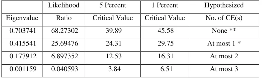
Furthermore, the regression results may be spurious due to no co-integration among the

series. To this end the Jhonson Co-integration test has been used. The likelihood ratios

statistic values are given in Table III (including no trend and no intercept) and in Table

IV (including both intercept and trend), which indicates the long-term relationship among

the variables of the study and rejects the hypothesis of no co-integration. Because most of

the absolute values of the LR ratios are greater than their relevant critical values.

Table III Johansson Co-integration test results including no intercept and no trend

Likelihood 5 Percent 1 Percent Hypothesized

Eigenvalue Ratio Critical Value Critical Value No. of CE(s)

0.703741 68.27302 39.89 45.58 None **

0.415541 25.69476 24.31 29.75 At most 1 *

0.177912 6.897352 12.53 16.31 At most 2

0.001159 0.040593 3.84 6.51 At most 3

Table IV Johansson Co-integration test results including both intercept and trend

Likelihood 5 Percent 1 Percent Hypothesized

No. of CE(s) Eigenvalue Ratio Critical Value Critical Value

0.765373 93.96282 62.99 70.05 None **

0.449030 43.22127 42.44 48.45 At most 1 *

0.383189 22.35862 25.32 30.45 At most 2

0.144120 5.446866 12.25 16.26 At most 3

*(**) denotes rejection of the hypothesis at 5%(1%) significance level L.R. test indicates 2 cointegrating equation(s) at 5% significance level

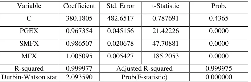
Regression results with TEX as dependent variable while PGEX, SMFX and MFX are as

independent variables are given in Table V. The results indicate that 1% increase in the

exports of primary commodities brings 0.97% increase in total exports in Pakistan.

Similarly, 1% increase in the exports of semi-manufactures leads to increase total exports

by 0.99%. On similar pattern, 1% increase in the exports of manufactured goods leads to

increase total exports by 1%. The coefficients of all the explanatory variables are

statistically significant at both 5% and 1% level of significance. The model is also best

fitted as indicated by the high value of R-squared (0.999) and adjusted R-squared (0.999),

showing that the included explanatory variables are entirely responsible for changes in

total exports in Pakistan.Durbin-Watson value (2.09) suggests that there is no problem of

autocorrelation.

Table V Regression results of export function

Variable Coefficient Std. Error t-Statistic Prob.

C 380.1805 482.6517 0.787691 0.4365

PGEX 0.967354 0.045156 21.42226 0.0000

SMFX 0.986507 0.020678 47.70881 0.0000

MFX 1.005095 0.005427 185.2053 0.0000

R-squared 0.999977 Adjusted R-squared 0.999975

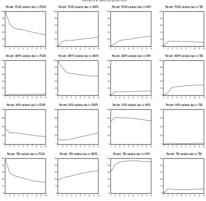
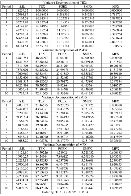
Table VI and figure 1 depicts the values of variance decomposition of the four variables,

showing how the variance of each one of the series is decomposed during a period of ten

years. The first group of columns in table VI is referred to total exports (TEX). Those

values of standard errors that total exports explain by itself lies between 83% to 100%

with values declining slowly. PGEX is the second variable explaining most of the

variation in TEX ranging from 9.3% to 13.1%. SMFX variation ranges from 0.24% to

0.18% and MFX explaining 3.78% to 3.10% variation in TEX.

On similar pattern, variances decomposition values of PGEX, SMFX and MFX are given

in Table VI and Fig 1.

0 2 0 4 0 6 0 8 0 1 00

1 2 3 4 5 6 7 8 9 1 0

Percent PGEX variance due t o PGEX

0 2 0 4 0 6 0 8 0 1 00

1 2 3 4 5 6 7 8 9 1 0

Percent PGEX variance due t o SMFX

0 2 0 4 0 6 0 8 0 1 00

1 2 3 4 5 6 7 8 9 1 0

Percent PGEX variance due t o MFX

0 2 0 4 0 6 0 8 0 1 00

1 2 3 4 5 6 7 8 9 1 0

Percent PGEX variance due t o TEX

0 2 0 4 0 6 0 8 0 1 00

1 2 3 4 5 6 7 8 9 1 0

Percent SMFX variance due t o PGEX

0 2 0 4 0 6 0 8 0 1 00

1 2 3 4 5 6 7 8 9 1 0

Percent SMFX variance due t o SMFX

0 2 0 4 0 6 0 8 0 1 00

1 2 3 4 5 6 7 8 9 1 0

Percent SMFX variance due t o MFX

0 2 0 4 0 6 0 8 0 1 00

1 2 3 4 5 6 7 8 9 1 0

Percent SMFX variance due t o TEX

0 2 0 4 0 6 0 8 0

1 2 3 4 5 6 7 8 9 1 0

Percent MFX variance due t o PGEX

0 2 0 4 0 6 0 8 0

1 2 3 4 5 6 7 8 9 1 0

Percent MFX variance due t o SMFX

0 2 0 4 0 6 0 8 0

1 2 3 4 5 6 7 8 9 1 0

Percent MFX variance due t o MFX

0 2 0 4 0 6 0 8 0

1 2 3 4 5 6 7 8 9 1 0

Percent MFX variance due t o TEX

0 1 0 2 0 3 0 4 0 5 0

1 2 3 4 5 6 7 8 9 1 0

Percent TEX variance due t o PGEX

0 1 0 2 0 3 0 4 0 5 0

1 2 3 4 5 6 7 8 9 1 0

Percent TEX variance due t o SMFX

0 1 0 2 0 3 0 4 0 5 0

1 2 3 4 5 6 7 8 9 1 0

Percent TEX variance due t o MFX

0 1 0 2 0 3 0 4 0 5 0

1 2 3 4 5 6 7 8 9 1 0

Percent TEX variance due t o TEX

Va ri a n c e De c o m p o s i ti o n

Table VI Values of the variances decomposition

Variance Decomposition of TEX:

Period S.E. TEX PGEX SMFX MFX

1 18259.32 100.0000 0.000000 0.000000 0.000000

2 25094.85 86.68458 9.288366 0.245289 3.781761

3 30163.58 86.61341 10.27218 0.226542 2.887865

4 35227.97 87.23794 10.18558 0.179262 2.397220

5 41148.96 86.94966 10.67850 0.133095 2.238748

6 47717.18 86.28204 11.36530 0.105782 2.246884

7 54782.31 85.55978 11.95579 0.097166 2.387264

8 62652.44 84.91816 12.39766 0.112508 2.571674

9 71428.95 84.25025 12.79103 0.142011 2.816701

10 81144.54 83.57158 13.14184 0.182046 3.104535

Variance Decomposition of PGEX:

Period S.E. TEX PGEX SMFX MFX

1 4781.751 48.95997 51.04003 0.000000 0.000000

2 6433.748 57.38482 30.36011 0.639148 11.61593

3 7311.705 62.29014 26.31264 0.495457 10.90176

4 7576.001 63.15232 24.99675 0.531239 11.31970

5 7960.969 65.83491 23.01880 0.555187 10.59110

6 8452.606 68.07865 21.52463 0.517305 9.879414

7 8908.315 69.18505 20.79172 0.475893 9.547334

8 9425.898 70.59508 19.92864 0.465564 9.010717

9 10036.44 71.89468 19.14508 0.459903 8.500338

10 10735.14 72.91603 18.53249 0.461251 8.090222

Variance Decomposition of SMFX:

Period S.E. TEX PGEX SMFX MFX

1 3703.173 21.46555 16.22020 62.31425 0.000000

2 5944.012 43.74351 18.43376 32.21773 5.605004

3 7620.185 33.14018 23.28134 23.05716 20.52133

4 9135.734 36.68694 21.84490 20.49156 20.97660

5 10567.97 38.84114 20.85234 17.83043 22.47610

6 11892.07 39.58045 20.24935 16.13129 24.03891

7 13168.42 41.07721 19.51060 14.93964 24.47254

8 14382.38 42.16697 18.97908 13.94103 24.91292

9 15548.34 43.10910 18.55014 13.16266 25.17809

10 16685.29 44.05778 18.17979 12.51048 25.25195

Variance Decomposition of MFX:

Period S.E. TEX PGEX SMFX MFX

1 14121.80 94.79226 1.289024 3.228032 0.690685

2 16930.27 84.24164 7.896125 6.798940 1.063298

3 20235.84 85.38635 6.637798 5.736808 2.239047

4 24000.61 86.86299 6.404671 4.811484 1.920855

5 28116.36 87.23508 7.468538 3.888298 1.408082

6 32885.80 87.53913 8.412174 3.018421 1.030279

7 38221.99 87.55922 9.301531 2.315824 0.823430

8 44324.24 87.35849 10.11760 1.743282 0.780629

9 51276.40 86.96601 10.84904 1.304543 0.880402

10 59098.99 86.42316 11.49372 0.983442 1.099679

CONCLUSION AND RECOMMENDATIONS

The facts and figures indicate that the major determinants of exports of Pakistan are

primary goods exports, semi-manufactures and manufactured goods’ exports. The results

indicate that 1% increase in the exports of primary commodities brings 0.97% increase in

total exports in Pakistan. Similarly, 1% increase in the exports of semi-manufactures

leads to increase total exports by 0.99%. On similar pattern, 1% increase in the exports of

manufactured goods leads to increase total exports by 1%. The planners are

recommended to make balance of trade favorable through increasing the exports of

primary goods, semi-manufactures and manufactured goods.

REFERENCES

Arize, A.C. (1999). “The demand for LDC Exports: Estimates from Singapore”. The

International Trade Journal, vol.13(4). Pp. 345-370.

Funke, M. and S. Holly (1992). “The Determinants of West German Exports of

Manufactures: An Integrated Demand and Supply Approach”, Weltwirtschaftliches Archive,128(3): 498-512.

Government of Pakistan, (2006-07). Statistical supplement, economic survey, finance

division, economic advisor’s wing, Islamabad.

Riedel, J., C. Hall and R. Grawe (1984). “Determinants of Indian Exports Performance in the 1970s”, Weltwirtschaftliches Archive,120(1): 40-63.

Sharma, K. (2001). “Export Growth in India: Has FDI Played a Role?”

at:http://www.econ.yale.edu/~egcenter/