The size of the underground economy in Japan

Munich Personal RePEc Archive

The size of the underground economy in

Japan

Kanao, Koji and Hamori, Shigeyuki

Kobe University, Kobe University

March 2010

Online at

https://mpra.ub.uni-muenchen.de/21562/

The Size of the Underground Economy in Japan

Koji KANAO

(Kobe University)

Shigeyuki HAMORI

(Kobe University)

Abstract

This paper empirically analyzes the size of the underground economy in Japan. The results show that (i) the size of the underground GDP peaked in the early 1990s but has been declining since; (ii) the underground economy reached its peak in around 1992, approximating 25% of nominal GDP; and (iii) two laws (the Act for the Prevention of Wrongful Acts by Members of Organized Crime Groups and the Act Regulating the Adult Entertainment Business, etc.) successfully worked to reduce the size of the underground economy.

1

1. Introduction

Tax evasion, drug dealing, gambling, fraud, prostitution, smuggling, and other economic activities that are hidden from public authorities and go unreported in official economic statistics are generally referred to as the "underground economy." The development of an underground economy can give rise to significant problems. To begin with, it creates difficulty in determining the status of activities in a real economy. If economic activities are examined using GDP statistics that do not account for the underground economy, then the actual size of the economy will be estimated to be smaller than that of the underground economy, and there is a strong possibility that macroeconomic conditions will be incorrectly assessed. The existence of an underground economy also results in a smaller tax base and tax revenues, and could contribute to fiscal deficits. Reflecting the importance of analyzing underground economies, much research (Gutmann 1978, Feige 1979, Gutmann 1979, Tanzi 1980, Feige 1982, OECD 1982, Tanzi 1983, Tanzi 1986, Hayashi 1985, and Kadokura 2001) has been carried out in this area, beginning with the pioneering work of Gutmann (1977).

Gutmann (1977) estimated the size of the underground economy on the basis of the following four hypotheses.

(1) All underground economy transactions are performed in cash.

(2) In the period in which the underground economy was nonexistent, its size for each year is established on the basis of the ratio of currency to demand deposit.1

(3) Excess currency demand is entirely due to the underground economy.

(4) The velocity of circulation is the same for both the underground and aboveground economies.

On the basis of these hypotheses, Gutmann (1977) concluded that underground economies are approximately 10% the size of their aboveground counterparts.

Feige (1979) advocated an analysis approach based on the perspective that the velocities of circulation can be different between aboveground and underground economies. Feige’s approach (1979) made use of Fisher’s equation of exchange to calculate the sizes of underground economies on the basis of the velocities of money circulation, demand deposits, and other exchange media.

Tanzi (1980) proposed an analysis approach based on the demand for currency equation. On the basis of the view that changes in currency demand are the result of underground economies, this approach builds on the one by Gutmann (1977). To estimate the demand for currency equation and to calculate the size of the underground economy, it uses a set of explanatory variables that includes variables considered to be related to the underground economy. Tanzi (1980) reported that underground economies are 2%~7% the size of aboveground economies.

2

Hayashi (1985) used the abovementioned three approaches to estimate the size of Japan’s underground economy. Using Gutmann’s (1977) approach, Hayashi estimated the underground economy to be approximately 4.4% the size of the aboveground economy in 1983. Applying Feige’s (1979) approach, it was estimated to be 58.8% the size of the aboveground economy in 1982. Moreover, using Tanzi’s (1980) approach, Hayashi estimated the underground economy to be 7.9% the size of the aboveground economy in 1983.

Kadokura (2001) also used the approach developed by Tanzi (1983) to analyze the size of Japan’s underground economy. He determined that the underground economy was approximately 4.5% the size of the aboveground economy in 1999 and that it had been shrinking after it reached its peak during the bubble era.

Estimating the sizes of underground economies has significant implications for policy management and economic forecasting. The purpose of this paper, therefore, is to expand on the analysis approach proposed by Tanzi (1983) and calculate estimates related to the size of Japan’s underground economy. This paper makes the following two contributions.

First, the paper takes into account the nonstationarity of time series—something that has not been done in previous research—and calculates estimates after performing unit root and cointegration tests. These steps allow for the calculation of statistically acceptable estimates. We used the unit root test propounded by Dickey and Fuller (1979) and the cointegration test proposed by Johansen (1988).

Second, to analyze the impact of legal measures on the underground economy, this paper uses dummy variables to capture the impact of two laws and integrates them in the model it employs to estimate and analyze the size of the underground economy. The two laws represented as dummy variables are the Act for the Prevention of Wrongful Acts by Members of Organized Crime Groups, which came into effect in 1992 and which was expected to have a great impact on the underground economy, and the Act Regulating the Adult Entertainment Business, etc., which underwent a major revision in 1984.

2. Basic Model

The basic model is composed of two equations: the demand for currency equation and an equation to calculate the size of the underground GDP. These two equations are given as follows.

0 1 2 3

4 5

log log( ) log( ) log( )

log( ) log( )

t t t t

t t t

C TG GN CY

WORK JR u

α α α α

α α

= + + +

+ + + (1)

(

)

(

)

t t t

C C UGDP GDP

M C C

−

= ×

3

where C_t represents funds; TG_t, taxes; GN_t, real income per capita; CY_t, the average

propensity to consume; WORK_t, an index for hours worked; JR_t, the unemployment rate;

t

u , an error term; UGDP, the underground GDP; GDP, nominal GDP; M1, the money supply; Cˆ, the currency demand forecast value (when the actual value is used); and *

t C , the

currency demand forecast value (when a value set for this study is used).

The demand for currency equation is represented by (1), and the equation to calculate the size of the underground GDP, by (2). At this point, it is important to bear in mind that the demand for currency in (1) is essentially the one to be used in the underground economy. In (2), the numerator and denominator of the second term on the right-hand side represent the demand for currency in the underground and aboveground economies respectively. M1 is used because of the hypothesis that only cash transactions are performed in the underground economy. The numerator to denominator ratio is taken to be the ratio of the underground economy to the aboveground economy, and multiplying this ratio by the GDP gives an estimate of the size of the underground GDP.

3. Data

Annual data for 1971–2007 were used for this study. The data sources are shown in Table 1. This study used two dummy variables to explicitly consider the impacts of two laws.

1_t

D is the dummy variable for the Act for the Prevention of Wrongful Acts by Members of

Organized Crime Groups, which came into effect in 1992.

0 1992 1 1 1992 t t D t < ⎧ = ⎨ _≥ ⎩ 2_t

D is the dummy variable for the Act Regulating the Adult Entertainment Business, etc., which underwent a significant revision in 1984.

0 1984 2 1 1984 t t D t < ⎧ = ⎨ _≥ ⎩

4

4. Empirical Results

Taking into account the nonstationarity of variables, we used the dynamic ordinary least squares (DOLS) approach proposed by Stock and Watson (1993) to estimate (1). This approach, represented in (3), produces estimates by adding lead and lag differences for each explanatory variable.

1 1

1 1

log log( ) log( ) log( ) log( )

log( log( ) log( ) log( ) 1 2

K K

t t t i t t i

i i

K K

t t i t t i

i i

t t t

C TG TG GN GN

WORK WORK JR JR

D D u

− −

=− =−

− −

=− =−

= + Δ + + Δ

+ + Δ + + Δ

+ + +

∑

∑

∑

∑

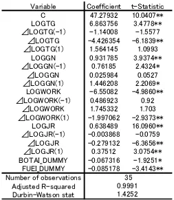
Given the small sample size, K in (3) was set as 1. Empirical results based on (3) are given in Table 2. As these results clearly show, the coefficients of each explanatory variable are statistically significant at the 5% level.

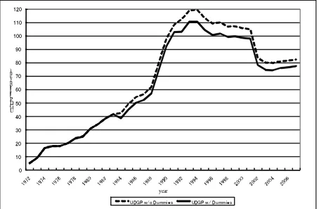
Having established the above, the size of the underground economy was calculated using (2). The results are presented in Figure 1, wherein the solid line indicates the size of the underground economy with explicit consideration of the dummy variables, while the wavy line indicates the size of the underground economy without consideration of the dummy variables. The difference between the two shows the suppressive impact of the two laws on the underground economy. Figure 1 clearly shows that the size of the underground economy peaks in 1993 when the dummy variables are considered, and in 1994 when they are not considered. Furthermore, the underground economy is shown to be at its peak at 120 trillion yen when the dummy variables are not considered, and at 111 trillion yen when they are considered. At these levels, the underground economy is estimated at approximately 25% of the nominal GDP. The suppressive impact of the two laws on the size of the underground economy was at its highest in 1992.

5. Concluding Remarks

Tax evasion, drug dealing, gambling, fraud, prostitution, smuggling, and other economic activities that are hidden from public authorities and go unreported in official economic statistics are generally referred to as the "underground economy." For this paper, data for 1971–2007 were used to estimate the size of Japan’s underground economy.

5

OLS approach. Second, it considers the impact of laws on the underground economy by including two dummy variables in the model it employs for estimating and analyzing the size of the underground economy. One variable is for the Act for the Prevention of Wrongful Acts by Members of Organized Crime Groups, implemented in 1992, and the other is for the Act Regulating the Adult Entertainment Business, etc., revised in 1984.

Empirical results indicated that the size of the underground GDP peaked in the early 1990s and has been declining since; this finding is consistent with that by Kadokura (2001). However, this study also estimates the underground economy to have reached a maximum size, approximating 25% of the nominal GDP, a scale much greater than that estimated by Kadokura (2001). Furthermore, the results of this study showed that the two laws referred to above contributed toward reducing the size of the underground economy.

References

Dickey, D.A. and W.A. Fuller (1979) “Distribution of the Estimators for Autoregressive Time Series with a Unit Root” Journal of the American Statistical Association74, 427-31. Feige, E.L. (1979) “How big is the irregular economy?” Challenge22, 5-13.

Feige, E.L. (1982) “A New Perspective on Macroeconomic Phenomena. The Theory and Measurement of the Unobserved Sector of the United States Economy: Causes, Consequences and Implications” in International Burden of Government by M. Walker, Ed., Fraser Institute: Vancouver, 112-136

Hayashi, H. (1985) Measurement of the Underground Economy, Statistical Data Bank.

Stock, J.H. and M.W. Watson (1993) “A Simple Estimator of Cointegrating Vectors in Higher Order Integrated Systems” Econometrica61, 783-820.

Johansen, S. (1988) “Statistical analysis of cointegration vectors” Journal of Economic Dynamics and Control12, 231-254.

Organisation for Economic Co-operation and Development (1982) The Hidden Economy and the National Accounts. Paris: OECD Occasional Studies.

Gutmann, P.M. (1977) “The subterranean economy” Financial Analysts Journal34, 26-27. Gutmann, P.M. (1978) “Are the unemployed, unemployed?” Financial Analysts Journal34,

26-29.

Gutmann, P.M. (1979) “Taxes and the supply of national output” Financial Analysts Journal

35, 64-66.

Cagan, P. (1958) “The demand for currency relative to the total money supply” The Journal of Political Economy66, 303-328.

Kadokura, T. (2001) “Time series analysis of the size of Japan’s underground economy and comparisons among Japan’s prefectures” Japan Center for Economic Research, http://www.jcer.or.jp/academic_journal/jer/PDF/46-8.pdf.

6

1930–1980” IMF Staff Papers30, 283-305.

7

Table 1 Source of Data

Variable Source

Cash Currency Bank of Japan

Tax

Household Disposable Income Nominal GDP

Real GDP

Nominal Final Expenditure of Household

Cabinet Office, Government of Japan

Population Ministry of Internal Affairs and Communications Index of Hours Worked

8

Table 2 Empirical Results of Dynamic OLS

Note:  *Significant at the 5% level, **Significant at the 1% level.

Variable Coefficient t-Statistic

C 47.27932 10.0407**

LOGTG 6.863756 3.4778**

⊿LOGTG(-1) -1.14008 -1.5577

⊿LOGTG -4.426354 -6.1839**

⊿LOGTG(1) 1.564145 1.0993

LOGGN 0.931785 3.9374**

⊿LOGGN(-1) 0.76185 2.4324*

⊿LOGGN 0.025984 0.0527

⊿LOGGN(1) 1.446208 2.2069*

LOGWORK -6.55082 -4.9860**

⊿LOGWORK(-1) 0.486923 0.92

⊿LOGWORK 1.745332 1.703

⊿LOGWORK(1) -1.997062 -2.9373**

LOGJR 0.638489 16.0960**

⊿LOGJR(-1) -0.003868 -0.0759

⊿LOGJR -0.279132 -6.3656**

⊿LOGJR(1) 0.37512 3.0754**

BOTAI_DUMMY -0.067316 -1.9251*

FUEI_DUMMY -0.085178 -3.4143**

Number of observations Adjusted R-squared Durbin-Watson stat

9

0 10 20 30 40 50 60 70 80 90 100 110 120

U G D P (t ri ll io n y en )

year

UDGP w/o Dummies UDGP w/ Dummies