Munich Personal RePEc Archive
Breeding Ones’ Own Subprime Crisis:
The effects of labour market on financial
system stability
Daras, Tomasz and Tyrowicz, Joanna
University of Warsaw, National Bank of Poland
2009
Online at
https://mpra.ub.uni-muenchen.de/15202/
Breeding Ones’ Own Subprime Crisis
The effects of labour market on financial system stability∗
Tomasz Daras
University of Warsaw
National Bank of Poland
Joanna Tyrowicz
University of Warsaw
National Bank of Poland
November, 2008
Abstract
In this paper we take a simulation approach towards household budgets survey, analysing the impact of changes in labour market status of household members on the ability of this household to service the mortgage payments.
Using the current status as benchmark, we performed simulations using stylised facts about labour market evolutions. Households with mortgage are characterised by higher activity rates and lower unemployment rates than demographically comparable households without a credit. While these are typical preconditions for the credit approval decision, this state of matters may not necessarily persist throughout the entire mortgage service period. Firstly, labour market conditions may worsen in general, comprising the credit takers together with the rest of the population. Alternatively, credit takers may undergo employment experience in the same way as other labour market participants. Consequently,
we performed analyses along two scenarios: (i) households with mortgages will gradually become alike the demographically comparable group in terms of employment performance; and (ii) recognising the fact that debtor households members may exert potentially higher effort in maintaining labour market status we model the effects of general employment outlooks deterioration. We use labour force survey data to obtain the probabilities of changing the individual labour market status, while we resort to propensity score matching techniques to provide adequate benchmark for the changes among creditors with relation to general population.
In the simulations we find the share of creditors loosing liquidity with the change in the labour market status and the implied burden to the financial sector stability.
Key words: financial sector stability, mortgages, labour market
JEL Codes: G21, C15, R20
∗Authors would like to thank Micha l Gradzewicz, Jacek Laszek, Ryszard Kokoszczy´nski, Tomaszk Michalak and Zbigniew
1
Introduction
In most theoretical approaches, credit worthiness is evaluated basing on ones’ likelihood to maintain the future burden of repayments. The origin of riskiness comes from the fact future liquidity of creditors remains unknown at the time of credit approval. For mortgages, it has been frequently argued in the literature, that scoring models can help to partly alleviate this problem by allocating potential clients differentiated probability of becoming delinquent in the credit horizon by using the proxies of demographic status, educational attainment and subsequently labour market prospects, (Wagner 2004). In principle, these models evaluate the future earnings using a Mincerian approach. On the other hand, in transition economies one observes large swings in the unemployment rate - in the case of Poland the movement from 10% to 20% and back to 10% thresholds was observed over less than a decade, which makes it very difficult to evaluate individual future labour market prospects basing on a current employment status.
Consequently, one could pose a research question concerning the risk of observing a crisis similar to sub-prime breakdown in the US as a consequence of deterioration in the Polish labour market. We addresses this question by developing a simulation framework using individual households’ budgets data for 2007. We observe the liquidity of households burdened with a mortgage loan. We subsequently simulate future employment prospects of income earners in these households using adapted labour force survey data.
Naturally, creditors differ from the population at large in terms of labour market situation - they are more active and definitely more frequently employed. In the simulations, we attempted to comprise two competing approaches. The first assumes that credit takers will consistently experience significantly better employment prospects due to for example higher search effort. Therefore, their odds of loosing and finding jobs will evolve together with the market conditions, but starting from the currently observed, significantly higher levels of employment persistence (the likelihood to remain in employment) and find rate (the likelihood of finding new employment). To this end we used LFS data for 1999-2004 period, which observed doubling of the general unemployment rate.
In the latter approach, we will not monitor the influence of exogenous labour market shifts that could occur for example because of the worsening growth prospects, but focus on endogenous changes in the labour market performance of the creditors. Namely, the simulated shock will comprise gradually equating the probabilities of flows into and out of employment with the comparable demographic groups. Therefore, in the second approach we provide analysis of what would be the effects of continuing with the current, relatively bold labour market conditions if one no longer subscribes to the view that credit takers are inherently different from the comparable non-borrowers in the population in terms of employment prospects. Our findings suggest that both simulated shocks will noticeably affect the ability of Polish households to service the mortgage payments. This impact - depending on the scenario - ranges from 63% to 78% increase in the number of delinquent households, while the volume of endangered credit may reach 3.6% to 10.4% of the 2007 outstanding mortgages.
The paper is structured as follows. In section (2) we briefly present the similarities and differences between current situation in Poland and outlooks in the US at the edge of sub-prime crisis emergence. Subsequently we present model setup in section (3). In section (1) we describe the data. Section (5) presents the results and implications for policy.
2
Literature review and context
To the best of our knowledge this type of research is unprecedented in the literature, while this paper contributes in two main ways. First of all, we use propensity score matching for recovered individual data from household budgets survey and originally individual data from labour force survey to obtain reliable benchmark for simulating the suggested scenarios. Secondly, we apply multi-agent systems approach (MAS) using micro-level data to arrive at macroeconomic estimates of financial system stability.
servicing burden, Barwell, Orla and Pezzini (2006), Simigiannis and Tzamourani (2006) and Faraqui (2006). Also for Swedish data this type of scrutiny was undertaken, using the so-called margin approach, which allows to define the liquidity of households taking into account servicing all debts and covering subsistence expenses, (Johansson and Persson 2006). However, both these approaches are backward looking in a sense that they analyse the indicators already experienced by the economy, while the projections are based on structural relationships between macro-level aggregates. We take the opposite angle using micro-level data for simulation exercises obtaining macroeconomic projections as outcome.
For Poland recently, Zajaczkowski and Zochowski (2007) used household budget survey data to perform stress-test for monetary and foreign currency shocks, while Osinski, Szpunar and Tymoczko (eds.) (2008) report the results of simulations in case of increased risk of becoming unemployed (unemployment rate growth by 4.7 percentage point, which is a conservative, ”pessimistic” projection). Both these studies reach the conclusion that Polish households liquidity is vulnerable to such exogenous shocks, but the stability of the financial system should remain unaffected.
Gorton (2008) analyses in detail the origins of the recent financial distress in the US describing how the banking system crisis emerged in the US from mortgage difficulties in the so-called subprime segment of creditors. However, the important conclusion from this text for any other economy experiencing construction and mortgage booms concerns the very nature of the so called ”subprime” credits. Namely, the terms ”sub-prime” and ”Alt-A” are not official designations of any regulatory authority or rating agency. Basically, the terms refer to borrowers who are perceived to be riskier than the average borrower because of a poor credit history. Sub-prime or Alt-A credits imply that loan-to-value ratio ranges between 60-70% and 100% (better rated mortgages usually do not exceed 80% thresholds). Home ownership for low income and minority households has been a long-standing national goal in the U.S. Sub-prime mortgages were an innovation aimed at meeting this target. The main issue to be confronted in providing mortgage finance for this unserved population was clearly that these borrowers are riskier.
Taking this standpoint as a benchmark one needs to identify the following similarities. Firstly, while indebtedness of Polish households is still low by OECD standards, credit action over the recent years has been spectacular. At the same time, it seems that the low rates of credits reported by the banks to the supervising authority as ”endangered” is much more a statistical artefact associated with rapidly increasing volume than a confirmation for increasing reliability of the client base.
Table 1: Polish mortgage market
2002 2004 2005 2006 2007 Outstanding mortgage credits [bln PLN] 44.0 50.5 58.9 84.3 128.7 - as % of households total outstanding debt [%] 22.3 21.8 23.6 28.0 34.3 Share of mortgage-secured loans in all real-estate related loans [%] 68.0 59.0 56.3 59.8 62.0 Share of private mortgage loans in all real-estate related loans [%] 60.0 87.0 84.5 86.3 83.9 Share of endangered credits in total credits [%] 14.0 17.2 13.3 9.4 6.3 Share of endangered mortgage credits in mortgage credits [%] 9.0 6.6 5,8 4.7 2.8 - in absolute values [bln PLN] 3.96 3.33 3.42 3.96 3.60
Source:Financial Supervision Commission
Taking the institutional perspectives, one needs to note that in general Polish banks in majority do not apply scoring models to evaluate creditors future ability to service debts [some reference here!!!]. Neither do they control for past income experience, relying solely on the type of employment contract and current job market situation. This state of matters may have similar consequences to the opening of credit possibilities to the so-called sub-prime debtors in the US. To be more precise, American lending institutions knew they were dealing with riskier clients than regularly, while Polish banks have little previous experience to benchmark the reliability of the current credit applicants. Nor is there a history of established mortgage contracts regularly served over the past 10-15 years, which balances the portfolio risk as a whole.
This trend has gradually expanded, widening the market for the mortgages, because future debtors ability to service loans was established based on de nomine interest rate and not de facto service burden. One could argue that the mortgages offered in Poland are subject to thorough regulation common for all EU countries. In addition, over the time constraints were imposed, forcing banks to evaluate creditworthiness based in the same information, regardless of the credit conditions currency denomination.
However, although these regulations might have lowered the risk of abusing currency and interest rate arbitrage opportunities by the borrowers, they are not able to counteract the market forces. For example, in the US mortgage market frequently used instruments were the so called hybrid adjustable rate mortgages (ARMs), where lower interest rate was guaranteed for two to three years out of the thirty year period of credit duration, while creditors were allowed to roll over the debt to subsequent ARMs (the so-called ”2/28” and ”3/27”)1. Looking at the Polish mortgage portfolio, vast majority has floating interest rate
benchmark (WIBOR or LIBOR), while additional source of risk is introduced by the exchange rates since approximately 70% of mortgages is denominated in foreign currency (swiss francs, euro and yens). Therefore, from the current average interest rate on mortgage, the increase of the burden could result easily from Polish zloty depreciation and/or increase in LIBOR. As we discussed earlier, Zajaczkowski and Zochowski (2007) demonstrate that the household liquidity effects of these exogenous shocks are likely to be considerable, but financial system stability should remain solid. We attempt to verify these results using micro-level simulations relying on behavioural relationships. Recent years have forcefully shown that a transition economy like Poland is prone to observe large swings in labour market outlooks with the number of employed increasing by almost two million over a period of just two years.
3
Model
Approaching this problem involves developing a framework of interaction between a trajectory of labour market status and household liquidity. Consider for simplicity one household member earning in a house-hold. His/her labour market status is a stochastic process with two possible states: Efor employment and
Nfor nonemployment. The future status is randomly allocated between these two states, either by changing the status (flows from employment to non-employment as well as from non-employment to employment) or by maintaining it. Depending on status in time t−1, the situation in time tis drawn from a distribution ΩE for transitions within employment as status at time t−1 or ΩN for nonemployment. Namely, each
individual faces a typical Bellman type function of
Vi
t = (ωt−ct) +βEt[πi,tVti+1+ (1−πi,t)Vti+1]
_
i=e, n (1)
whereπe,tdenotes the probability of remaining in employment andπn,tdenotes the probability of remaining
in nonemployment. Naturally, the transition rates are given by the compliments these values,i.e. of 1−πe,t
and 1−πn,tfor loosing and finding employment, respectively2. We simulate this equation and compare the
obtained values with the subsistence expenses for the household increased with the mortgage installments reported earlier by the household. This way we obtain a measure of interest for further analysis, residual income.
Household survey data suffer from many well known shortcomings, including underreporting. In ad-dition, individual credit characteristics like currency, duration and age of credit remain unknown, which makes it impossible to include a la stress-test approach in this study. For subsequent analyses we take the reported values as given and only observe the effects of changes inπi,t parameters on the households’
liquidity and at the end of the simulations - the aggregate threat to the financial sector.
1
In fact, although these mortgages originated with low fixed rates, they could have been reset semi-annually based on an interest-rate benchmark or the current going rate after the first two to three years period. For many holders, payments soared effectively 15%-20%per annumand thus became unaffordable. By 2004, 90% of subprime loans qualified as these type ARMs.
2
3.1
Labour market transitions
[image:6.595.93.518.232.460.2]The empirical transition probabilities are obtained from empirical model as suggested by Mortensen and Pissarides (1994) and developed recently by Shimer (2008). For the purpose of clarity, we only have two states of the labour market status: employment and non-employment. Although flows into inactivity are considerable in Poland, cfr Figure (1), we assume that having a mortgage is a strong incentive to maintain activity in the labour market. Therefore, we take the current aggregate inactivity rate as the maximum possible and keep it constant throughout the simulation exercise3.
Figure 1: Source: Labour Force Surveys, 1995-2007
Consequently, implicitly any unemployment in our model is involuntary and any shock we model is a consequence of changes in labour demand and not variability of household labour supply decisions. We de-cided to confine to employment and non-employment, because, from the perspective of households’ income, unemployment benefit and social assistance are comparable, while the key issue concerns the ability to earn income sufficient to service mortgage payments.
In principle, flows between states should be described by two independent equations:
Et = (1−πN, t)Nt−1+πE, tEt−1−(1−πE, t)Et−1 (2)
Nt = πN, tNt−1+ (1−πE,t)Et−1−(1−πN,t)Nt−1, (3)
which can subsequently be solved forπNt andπEt. Consequently, using labour force survey data one can
establish these actual values for a chosen reference period.
Unfortunately, in practice there are two considerable difficulties with establishing relevant empirical values for these parameters. First of all, there exists a large discontinuity problem when one uses actual Polish labour force data (large variability of estimators due to three significant changes in labour force survey methodology). Therefore, actual data for period 1998-2001 (recent deterioration in labour market outlooks) have been smoothed. Secondly, creditor households differ noticeably from general population. Namely, they are more frequently employed and experience lower risk of being unemployed or inactive, cfr Figure (??). Imposing the values characteristic for the whole population would impose the risk of excessive
3
job loss hazard in the simulation. However, it would be difficult to justify any arbitrary adjustments in these transition rates.
To overcome this former difficulty we have chosen the following empirical strategy. Firstly, we have separated the labour market status (and earnings) for each of the household members separately across the households. This allows as to treat household members as individual labour market participants and compute household revenues as a sum of individual earnings. The procedure for the separation is described in the coming subsection.
The second step was to use propensity score matching technique to obtain relevant labour market trajectories from the labour force survey. Namely, we used demographic, educational and geographical characteristics to match members of creditor households obtained through household budgets survey with individuals from labour force survey. For each of the points in time over the analysed period we have obtained comparable unemployment, inactivity and employment rates, which provided reliable benchmark for simulations. This procedure is described in the following subsection.
3.2
Moving from household to individual data
Household budgets survey data do not contain detailed information on the revenues of individual household members from each source of income, only data aggregated at the household level are available. In order to model the situation of individuals in the labor market and the corresponding revenues we distribute house-hold income among members mainly on the basis of primary and secondary income source for each person, which are reported separately. For example, for a two member household data set contains information about household revenue and sources of revenue as well as type of occupation for each member. Therefore, one can attribute the revenues from a certain type of income to a person that reported having this type of income source.
In case two or more individuals having the same source of income additional data were used to separate revenues: education, gender, person number as well personal income distribution by gender and education. This procedure was applied to (i) wage income, (ii) self-employment income, and (iii) benefits and transfers.
3.3
Creating reliable counterfactual
Propensity score matching is a relatively new technique. It is typically applied to estimate causal treatment effects (eg. the effectiveness of labour market policies, pharmaceutical research or profitability of particular marketing solutions or the effect of institutions on economic development). Caliendo and Kopeinig (2008) discuss in detail recent development as well as guide through the process of adequate construct of this approach. The critical element in propensity score matching lies in the conditional independence assumption construct. In other words, for the reliability of the results it is important that the selection is solely based on observed characteristics and that all variables that influence belonging to the shadow economy and potential earnings are simultaneously observed. In practice it implies that there should be no other sources of systematic (i) selection and (ii) outcome.
With propensity score matching, the quality of estimation depends much on the data availability. In the case of this study, the pool for matching (the size of the control sample in the relation to the size of the analysed sample) is relatively large, so there is no need for sampling with replacement. We apply kernel estimates of propensity scores with the nearest neighbour matching, following Heckman, Ichimura, Smith and Todd (1998). Alternatively, we could have used the oversampling technique. However, the choice of the oversampling magnitude is always arbitrary, while tenfold oversampling (as feasible in our sample) should not differ from the kernel approach in terms of statistical quality.
Rubin (1983).
[image:8.595.88.532.267.466.2]In particular, we have performed two matching procedures. In the first version for each continuous variable we have created categorical variable, subsequently dummies for each category (both on the new variables and in the initially categorical ones) and subsequently created interaction terms between these dummies. Propensity score matching was performed based on these interactions. In the second version we kept the originally continuous variables and included them directly, enriched with the standard interactions (education and gender, age and gender, age and place of residence, education and place of residence). In both attempts the propensity score procedure failed to match people with below vocational education among the creditors. In terms of other variables, the matching procedure exhibited more than satisfactory properties4. The labour market trajectories over the period 1998-2003 are depicted in Figure (2).
Figure 2: Labour force survey data matched with individuals recovered from household budgets survey data
These results clearly demonstrate two facts. First of all, statistical twins to the creditors observe through-out the entire period considerably lower unemployment rates. Secondly, they too experience worsening of the employment prospects, while the relevant observed unemployment rate doubled over the period of 1999-2004. Consequently, even when the employment prospects are good, the differential between the reported unemployment rate among the creditors and matched ”statistical twins” may gradually disappear, which constitutes our first scenario of analysis. Alternatively, if one subscribes to the view that there still persists significant unobserved heterogeneity between creditors and ”statistical twins”, the employment prospects may worsen with time, which gives support to our second scenario.
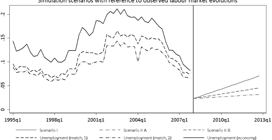
The question is naturally, which of while with the worsening of the unemployment prospects should be considered. First of all, the first scenario involves imposing a considerable shock (unemployment rate increase from 2.6% to 7.2%) as depicted by Figure (3). This may indeed be a pessimistic scenario if one considers that from the bottom to the top of the national unemployment rate the change was slightly above twofold. Therefore, it seems reasonable to consider also the alternative scenario. Intuitively, it corresponds to the situation coined as ”when water goes up, all ships go up”. However, to define the benchmark we differentiate between deterioration to the level of unemployment consistent with the current National Bank of Poland projection (national of 12% with the corresponding matched of 8,8%) and deterioration to the highest possible unemployment rate (national of 21,2% and matched of 14%). These two cases are respectively scenarios II A and II B. The simulation assumptions are presented at Figure (3).
4
Figure 3: Simulation scenarios
3.4
Simulation setup
In order to benchmark the simulation outcomes, at the first stage steady state transition probabilities were created. The steady state characteristic refers to a situation in which within 20 periods of simulations flows into and out of employment for all income earners were comparable. This means that essentially under the initial calibration the number of households able to service the debts is not affected despite random allocations of events corresponding to the labour market status change.
The simulation procedure is described by the following steps:
1. labour market status of each individual at timet is determined;
2. probability of change is randomly assigned to each individual;
3. selected probability is compared to empirically derived thresholds (there are two separate distribu-tions for E and N derived from labour market transidistribu-tions discussed in the above secdistribu-tions, threshold probabilities differ between scenarios and have been calculated separately for different gender and education groups)
(a) if flow from E to N occurs (individual looses employment), earnings of this individual are sub-tracted from the household reported revenues;
(b) if the flow from N to E occurs, individual obtains employment and a randomly selected income is added to the household reported revenues (distribution of income is recovered from original data of creditor households);
(c) if individual remains in either of the states, the financial situation of the household remains as in the previous period;
4. subsequently we subtract mortgage payment and subsistence living expenses relevant to the size of household;
6. we compute the residual income at each point in time;
7. we continue with this procedure for 20 subsequent periods (equivalent to 5 years);
8. we repeat the procedure 500 times.
Step (5) was necessary, because already data for 2007 suggest that almost one out of five households cannot service their mortgage. This may be a consequence of either income underreporting or alternative family (as opposed to household) strategies. For example, servicing mortgages may be supported by other family members (inter-generational transfers), who do not constitute the reporting households. Therefore, in the simulations we use the current situation as benchmark.
In addition to these calculations we have also introduced a policy instrument, i.e. in case of loosing employment individuals may obtain a benefit of 500 PLN (its size corresponds to unemployment benefit and social assistance benefit), maintained for four consecutive periods (in case individual does not find employment within the time span).
4
Data
Polish households survey data show that at the end of 2007 3.6% of households included mortgage repay-ments in their monthly expenses. If one took the aggregate data from financial system reports, with an additional assumption of approximately one credit per household, approximately 7.6% households should report mortgage repayments. Consequently, it seems that approximately a half of mortgages is missing from the household survey data, which may undermine their relevance. On the other hand, survey data are representative for location and size of the household, while housing loans tend to cluster in large agglomera-tions and among certain demographic groups of households. The comparison of demographic characteristics between creditor and non-creditor households is presented in Table (2).
Data suggest that the majority of the credits appears in young households (under 35 years), with median at exactly this age threshold. Also, mortgage repayment is inversely correlated with age, with younger creditors burdened with more credit. Consequently, the ”missing” mortgages should rather be perceived as a consequence of over-representation of the young, well educated households in the creditors group when compared to the nation-wide benchmark. Therefore the observed discrepancy does not necessarily imply data unreliability. This assertion is further corroborated if average size of credit is compared. Based on the reported value of monthly mortgage installments we have computed the approximate size of credit in order to compare the obtained result with the general data on mortgage market. Both in aggregate terms and based on household data the average credit size amounts to approximately PLN 100 000.
Using household survey for 2007 we have identified 1300 households who report mortgage repayments out of approximately 37 000 taking part in the survey. These households are populated by 2 177 working individuals, 69 unemployed and 887 inactive. For the purpose of simulations, we keep constant throughout the analysis the number of 887 individuals and only manipulate the number of unemployed. Moreover, because there were very few households with more than two income earning individuals, we treated these revenues as ”autonomous” and the labour market status of these household members is not modeled.
When using household level data one typically faces great difficulty following from underreporting of wage income and/or other revenues. Based on national accounts one could consider rescalling the household reported revenues by a certain average ratio that corresponds to the differential observed between house-holds’ survey reporting and data recorded within national accounts. These scaling factors differ significantly depending on the type of income ranging from 1.26 for retirement benefit as the main source of income to as much as 4.74 for self-employed. Therefore, relying on household declaration in determining their liquidity is bound to be troubled by reliability of the estimates. Therefore, we have attempted to verify to what extent the underreporting provides an information constraint in this study.
Table 2: Creditors and general population of households
Creditors General population
No. of households 1 321 3,53% 37 366 100%
No. of households (weights adjusted) 512 378 14 164 0005
No of people (sample) 4 177 100% 111 992 100% No. of people (weights adjusted) 1 580 045 53 329 132
No. of adults 3 134 75% 914 23 82%
No. of adolescent 1 043 25% 20 569 18%
No. of working 2 177 52% 47 076 42%
No of not-working
No. of unemployed 69 2% 3 485 3%
No. of inactive 887 21% 40 768 36%
Place of residence
Large city (above 500 tho) 24 14,5
City (200 - 500 tho) 13,5 11
Small city (100 - 200 tho) 9,8 8,9
Town (20 - 100 tho) 22,9 20,2
Small town (under 20 tho) 11,1 12,6
Rural areas 18,8 32,8
Household structure
Married, no children 17,1 15
Married, 1 child 11,2 24,8
Married, 2 children 11,2 21,5
Married, 3 and more children 4,9 5,9
Single parent 2,3 2,7
Married with children and other dependent 10 7,2 Single parent with children and other dependent 2,8 1,4
Other relatives with children 1,3 0,4
Single 24,8 12,8
Other 14,4 8,1
Household income (PLN) Mean Median Mean Median Young (under 35), tertiary education 5 493 4 413 4 104 3 343 Young (under 35), below tertiary education 3 803 3 223 2 662 2 249 Above 35 years or age 4 332 3 533 2 537 2 095
Household equivalent income (PLN)
Young (under 35), tertiary education 2 907 2 361 2 256 1 845 Young (under 35), below tertiary education 1 756 1 469 1 227 1 008 Above 35 years or age 1 865 1 518 1 236 1 059
Income per household member (PLN)
Young (under 35), tertiary education 2 370 1 900 1 878 1 513 Young (under 35), below tertiary education 1 341 1 068 964 766 Above 35 years or age 1 488 1 199 1 045 900
Monthly installment (PLN)
Young (under 35), tertiary education 706 525 - -Young (under 35), below tertiary education 589 410 -
-Above 35 years or age 539 380 -
-Source:Household budgets survey data, 2007, own calculation
relative to the population. To this end, we have analysed other source of information about the household liquidity available from the survey.
4.1
Liquidity concerns of the households
The basic variable of interest in this study is the liquidity of the households. Namely, we calculated the residual revenue, i.e. funds at disposal after subtracting subsistence expenses for each household member as well as credit monthly instalments from the declared household revenue. Taking household situation in 2007 as a starting point one may be surprised to observe that already then on average 19.8% of the households cannot service debts. For young households (head under 35 years of age) this number is as high as 20.71% (for the reminder of the sample it is 18.54%), which implies one out of each five credits is not sustainable. This number is strikingly high, especially if one confronts it with relatively low default ratio observed in the economy.
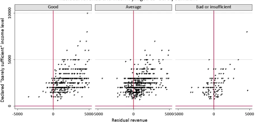
Figure 4: Declared preferred income and current liquidity, household survey data
the repayments. One observes that these two values (”barely sufficient” income andresidual revenue) are essentially closely correlated, while the link is not far from one-to-one. Naturally, as frequently in survey data, individual perceptions differ, while declared ”barely sufficient” income tends to be provided in rela-tively round numbers (which explains horizontal alignment of observations). Nonetheless, income reported by the households seems to be fairly consistent with the actual households’ perception of their financial situation. Consequently, we take the stand that even if actual value of revenue reported by the household is somewhat underreported, for credit taking households its level is at the very least consistent with the actual ”gap” declared by the household.
In addition to graphical presentation, we also compare the distributions of answers for the total sample and creditors. Namely, households are asked to evaluate their liquidity situation. We clearly observe that households with mortgage enjoy better situation than an average Polish household. However, if we inquire those with negative values ofresidual revenue, difficulties are more profound than on average in the population, Table (3).
Table 3: Delinquency and self-evaluation
How do you evaluate the liquidity situation of your household?
Not liquid Hardly Rather hardly Rather easily Easily Very easily Total
Delinquent 39 97 372 373 137 41 1,059
Liquid 28 54 142 33 5 0 262
Total 67 151 514 406 142 41 1,321
% delinquent 58,2% 64,2% 72,4% 91,9% 96,5% 100,0% 80,2% % liquid 41,8% 35,8% 27,6% 8,1% 3,5% 0,0% 19,8%
Source:Household budgets survey data, 2007, own calculation
Namely comparing the frequency of answers one obtains approximately 18.2% of creditor households declaring liquidity difficulties (answers from ”no liquidity” to ”some hardship”). This too is consistent with the earlier reported finding of 19.7% of households already unable to service the mortgage payments.
simula-tions both cases (corrected and raw income) are used. In our sample, a large share of households members report earnings from self-employment which leads to the difference in average scaling factor: it is 1.92 for the creditors whereas in population it amounts to 1.71.
5
Results
This section reports the results of the simulations performed 500 times over 20 periods. We have taken two perspectives to provide informative outcomes. First, we have observed the distributions of theresidual revenue, observing the percentile of the distribution for which households become delinquent under diverse scenarios. Second, we used these results to provide estimates of the threat to the stability of the financial system depending on a scenario.
All results are reported in two variants. Namely, in the simulations all individuals moving from employ-ment to non-employemploy-ment may obtain a benefit of 500 PLN (which is barely equivalent to the unemployemploy-ment benefit in Poland). However, calculating the residual revenue we implicitly assume that household only allocates to consumption the so-called subsistence minimum6. In the real world, however, it is likely that
the households experiencing the worsening of the financial situation will not be able to constrain previously higher consumption to this very low level. Therefore, one should consider the ”no instrument” scenario to refer to a case where the households allocate unemployment benefit entirely to consumption not facilitating mortgage servicing. Alternatively, ”instrument” scenario refers to a situation where the mortgage servicing has strict priority over consumption and delinquency is theactual household’s condition7.
[image:13.595.99.526.490.610.2]Table (4) reports the findings concerning the stability of the financial system. Comparing the annual change in credit volume between 2006 and 2007, Meluch and Wydra (2008) establish mean credit volume over 2007. Relying in this result we have established a benchmark for our calculations. Based on the properties of credits distribution with reference to currency of denomination as well as average value of one PLN of repayment in a typical credit we were able to uncover the estimate of an outstanding mortgage debt for the households reporting installment expenses. The average size of the credit in the sample is similar to the average size of the credit in the economy (approximately 100 000 PLN)8.
Table 4: Simulation results
With policy instrument No policy instrument
I II A II B I II A II B
Sum of credits (bln PLN) 128.7 128.7 128.7 128.7 128.7 128.7 The sum of endangered credits at t=0 (bln PLN) 20.0 20.0 20.0 20.0 20.0 20.0 Share of endangered credits 15.5% 15.5% 15.5% 15.5% 15.5% 15.5% Sum of endangered credits at t=20 (bln PLN) 28.1 24.4 25.8 29.6 25.4 27.0 Share of endangered credits 21.9% 19.0% 20.1% 23.0% 19.8% 21.0% Increase in endangered credits (bln PLN) 8.2 4.4 5.9 9.6 5.5 7.0 Ratio of residual revenue to monthly household expenses (average)
at t=0 -0,246 -0,246 -0,246 -0,246 -0,246 -0,246
at t=20 -0,392 -0,360 -0,372 -0,424 -0,386 -0,400
Change 0,146 0,114 0,126 0,178 0,140 0,155
Source:Own calculation based on household budgets survey data (2007)
Essentially, in the second scenario, as much as PLN 8.2 bln of outstanding mortgage credit may eventu-ally become unsustainable, while with the most optimistic scenario this number goes down to PLN 4.4 bln in the ”instrument” scenario (PLN 9.6 bln and PLN 5.5 bln in the ”no instrument” scenario respectively). If compared to the current credit boom, these numbers amount to 18.5%-26.3% of the credit action over 2007, (Meluch and Wydra 2008). Importantly, these numbers follow from a relatively mild shock. The
6
It is defined annually by the Ministry of Labour and Social Affairs.
7
In practice this may be obtained by,e.g. transferring the unemployment or social assistance benefits to mortgage repay-ments directly by the state.
8
increase in the share of unsustainable credits only increases by 3.5 to 4.3 percentage points in scenario II A and (6.4 to 7.5 percentage point in the ”no instrument” version)9. In terms of households results are
[image:14.595.93.532.174.273.2]reported in Table (5).
Table 5: Results of the simulations
Mean percentile Standard deviation Maximum 3rd quartile Median 1st quartile Minimum
Steady state 0.18 - - -
-A: No policy instrument
Scenario I 0.25 0.001 0.28 0.26 0.25 0.24 0.23
Scenario II A 0.21 0.01 0.24 0.21 0.21 0.21 0.19
Scenario II B 0.23 0.01 0.25 0.23 0.23 0.22 0.21
B: With policy instrument
Scenario I 0.24 0.01 0.27 0.24 0.24 0.23 0.21
Scenario II A 0.20 0.01 0.22 0.21 0.21 0.20 0.18
Scenario II B 0.22 0.01 0.24 0.22 0.22 0.21 0.20
Source:Own calculation based on household budgets survey data (2007)
Table (4) already shows the percentile ofresidual revenuedistribution for which the value becomes neg-ative,i.e. the share of households who no longer can service the mortgage loans. However, this delinquency might be only marginal with reference to the revenues they have at disposal. Therefore, we have analysed the distributions properties, providing the value of negativeresidual revenue relative to the expenses com-prising the monthly mortgage installments10. Namely, the ratio is defined as a relation between residual
[image:14.595.109.520.414.548.2]revenue and the sum of subsistence expenses and mortgage monthly installments. We only analysed the negative values ofresidual revenues. Results are reported in Table (6)
Table 6: The ratio of residual revenue to monthly household expenses (only delinquent households)
Percentile Bottom 10th 20th 30th 40th 50th 60th 70th 80th Top 90th Benchmark -0.459 -0.348 -0.290 -0.246 -0.204 -0.155 -0.122 -0.082 -0.039
With instrument
Scenario I -0.851 -0.637 -0.493 -0.386 -0.307 -0.241 -0.178 -0.120 -0.065 Scenario II A -0.818 -0.578 -0.448 -0.347 -0.277 -0.221 -0.161 -0.110 -0.059 Scenario II B -0.843 -0.607 -0.468 -0.363 -0.289 -0.229 -0.168 -0.114 -0.061
No instrument
Scenario I -0.974 -0.743 -0.546 -0.424 -0.329 -0.260 -0.196 -0.128 -0.068 Scenario II A -0.909 -0.608 -0.463 -0.362 -0.291 -0.232 -0.172 -0.117 -0.064 Scenario II B -0.938 -0.643 -0.486 -0.381 -0.305 -0.243 -0.181 -0.121 -0.066
The reduction in ratio due to policy instrument
Scenario I 0.122 0.106 0.053 0.038 0.022 0.019 0.018 0.007 0.004 Scenario II A 0.091 0.030 0.015 0.015 0.013 0.011 0.010 0.006 0.005 Scenario II B 0.095 0.036 0.019 0.018 0.016 0.014 0.014 0.007 0.005
Source:Own calculation based on household budgets survey data (2007)
Visibly, the reduction in the ratio is most profound in the bottom end of the distribution, which suggests largest liquidity problems persist in lowest ratio households. In principle, this may include high income households with large mortgages as well as low revenue household with lower credits. However, the average value of installments in the bottom of the distribution is lower, which suggests the instrument will be particularly efficient in the case of poorer households. The reduction in the ratio may be as high as approximately 10% in this group. Nonetheless, the instrument as constructed for the purpose of these simulations, does not eliminate the threat to the stability of the financial system associated with labour market impact on households’ delinquency.
9
To some extent the large effect of a relatively mild shock is a consequence of the fact that the creditor households have lower number of members than on average, which implies that loosing one source of wage income is equivalent to loosing all sources of wage income (no diversification at the household level).
10
As declared earlier, throughout the analysis we assume the value of installments remains unchanged in real terms,i.e.
6
Concluding remarks
Subprime crisis which originated in the US spread to many countries via the financial integration links. Monetary and fiscal authorities in many countries ponder about the ways of immuning the economy to the spreading of the crisis. In this paper we attempted to test if using the household survey data -typically available in all the developed economies - one can actually evaluate a risk of breeding one’s own subprime crisis instead. We find that even with relatively small number of creditors (in the Polish economy only approximately 7.6% of households have a mortgage) the actually effects of deteriorating the financial situation among the debtors can be indeed sizeable.
We use simulations in order to observe the impact on household liquidity derived from two alternative scenarios. In the first, we explicitly model the deterioration of labour market status due to, for example, economic slowdown. In the latter, we observe the consequences of creditors gradually resembling their counterparts within respective subgroups of the population in terms of labour market performance. In both cases we find that even small changes in the employment persistence or unemployment risk can lead to considerable deterioration of households’ liquidity and therefore the financial stability of the whole mortgage market. Please note, that in simulation we do not allow for the bank intervention (e.g. selling of the property, relieving the monthly installments, etc.). Naturally, observing lowering ability to repay the debts bank may engage into cooperating with the clients on designing tailored solutions. On the other hand, having the large number of agents in the simulation, this model outcomes hold by the token of statistics. Finding future creditors with better labour market outlooks will not be statistically feasible if the assumptions of our model hold and the simulation scenarios are relevant.
There are few issues we did not cover in the model. Firstly, already in 2007 a large share of households would not be able to service mortgage payments - 20% for raw income data and 9% if income reported by the households was corrected using benchmark values obtained from the national accounts. This is at odds with endangered credit volumes reported by the banks - at the end of 2007 approximately 1% of credits, (Meluch and Wydra 2008). We seek the roots of this situation in the fact that many young creditors may actually benefit from the support of their families. Alternatively, some underreported employment (gray economy) may matter for the liquidity of the households. None of these issues may be tackled using household survey data, however.
References
Barwell, R., Orla, M. and Pezzini, S.: 2006, The Distribution of Assets, Income and Liabilities Across UK Households: Results From the 2005 NMG Research Survey,Technical report, Bank of England. Caliendo, M. and Kopeinig, S.: 2008, Some Practical Guidance For The Implementation Of Propensity
Score Matching,Journal of Economic Surveys22(1), 31–72.
Faraqui, U.: 2006, Are There Significant Disparities in Debt Burden Across Canadian Households? An Examination of the Distribution of the Debt Service Ratio Using Micro Data,Measuring the Financial Position of the Household Sector, Vol. 2, IFC Bulletin .
Gorton, G. B.: 2008, The Subprime Panic, NBER Working Papper 14398, National Bureau of Economic Research.
Heckman, J., Ichimura, H., Smith, J. and Todd, P.: 1998, Characterizing Selection Bias Using Experimental Data,Econometrica66(5), 1017–1098.
Johansson, M. W. and Persson, M.: 2006, Swedish Households’ Indebtedness and Ability To Pay – a Household Level Study,Measuring the Financial Position of Household Sector, Vol. 2, IFC Bulletin. Meluch, B. and Wydra, M.: 2008, Rynek finansowania nieruchomosci mieszkaniowych w Polsce - stan na
Mortensen, D. T. and Pissarides, C. A.: 1994, Job Creation and Job Destruction in the Theory of Unem-ployment,Review of Economic Studies61(3), 397–415.
Osinski, J., Szpunar, P. and Tymoczko (eds.), D.: 2008, Raport o stabilnosci systemu finansowego (report on the financial system stability), National Bank of Poland, semi-annual report. Frame 2, p. 43.
Rosenbaum, P. and Rubin, D.: 1983, The Central Role of the Propensity Score in Observational Studies for Causal Effects,Biometrika 70(1), 41–55.
Shimer, R.: 2008, The Probability of Finding a Job,American Economic Review 98(2), 268–73.
Simigiannis, G. T. and Tzamourani, P.: 2006, Greek Household Indebtedness and Financial Stress Results from Household Survey Data,Measuring the Financial Position of the Household Sector, Vol. 2, IFC Bulletin .
Wagner, H.: 2004, The Use Of Credit Scoring In The Mortgage Industry , Journal of Financial Services Marketing9(2), 179–183.